1
****************************************************;
2 ***
Example of Analysis of Covariance
***;
3 ***
Steel and Torrie (1980) example (pg.
424) ***;
4 ***
Analysis of three diet treatments on two ***;
5 ***
sexes, where X is the initial weight, ***;
6 ***
and Y is the weight gain in pounds. ***;
7
****************************************************;
8 OPTIONS
NOCENTER PS=256 LS=132 nodate nonumber;
9 DATA
HOGS; INFILE CARDS MISSOVER;
10
Title1 'Analysis of Covariance example from Steel & Torrie, 1980';
11
INPUT
PEN SEX $ RATION $ X Y;
12 CARDS;
NOTE: The data set WORK.HOGS has 30 observations and 5
variables.
NOTE: DATA statement used:
real
time 0.05
seconds
cpu time
0.05 seconds
12 !
RUN;
43 ;
44 PROC
PRINT DATA=HOGS; Title2 'Raw data listing'; RUN;
NOTE: There were 30 observations read from the data set
WORK.HOGS.
NOTE: The PROCEDURE PRINT printed page 1.
NOTE: PROCEDURE PRINT used:
real
time 0.04
seconds
cpu time
0.04 seconds
Analysis of Covariance example from Steel & Torrie,
1980
Raw data listing
Obs PEN SEX
RATION X Y
1 1
M a1
38
9.52
2 1
F a1
48
9.94
3 1
M a2
39
8.51
4 1
F a2
48
10.00
5 1
M a3
48
9.11
6 1
F a3
48 9.75
7 2
M a1
35
8.21
8 2
F a1
32
9.48
9 2
M a2
38
9.95
10 2
F a2
32
9.24
11 2
M a3
37
8.50
12 2 F
a3 28 8.66
13 3
M a1
41
9.32
14 3
F a1
35
9.32
15 3
M a2
46
8.43
16 3
F a2
41
9.34
17 3
M a3
42
8.90
18 3 F
a3 33 7.63
19 4
M a1
48
10.56
20 4
F a1
46
10.90
21 4
M a2
40
8.86
22 4
F a2
46
9.68
23 4
M a3
42
9.51
24 4
F a3
50
10.37
25 5
M a1
43
10.42
26 5
F a1
32
8.82
27 5
M a2
40
9.20
28 5
F a2
37
9.67
29 5
M a3
40
8.76
30 5
F a3
30
8.57
46
PROC
MIXED DATA=HOGS; CLASSES RATION SEX PEN;
47
TITLE2 'Analysis of Covariance Example';
48
TITLE3 'Design done in PROC MIXED without a covariable';
49
MODEL
Y = RATION|SEX / htype=1 3 DDFM=Satterthwaite;
50
random PEN;
51
LSMEANS RATION|SEX / ADJUST=TUKEY PDIFF;
52
ods
output diffs=ppp;
53
ods
output lsmeans=mmm;
54
ods
listing exclude diffs;
55
ods
listing exclude lsmeans;
56
run;
NOTE:
Convergence criteria met.
NOTE: The data
set WORK.MMM has 11 observations and 8
variables.
NOTE: The data
set WORK.PPP has 19 observations and 12
variables.
NOTE: The
PROCEDURE MIXED printed page 2.
NOTE:
PROCEDURE MIXED used:
real
time 0.22
seconds
cpu
time
0.22 seconds
57
%include
'C:\Program Files\SAS
Institute\SAS\V8\stat\sample\pdmix800.sas';
673
%pdmix800(ppp,mmm,alpha=.05,sort=yes);
Analysis of
Covariance example from Steel & Torrie,
1980
Analysis of
Covariance Example
Design done in
PROC MIXED without a covariable
The Mixed
Procedure
Model Information
Data
Set
WORK.HOGS
Dependent
Variable Y
Covariance
Structure
Variance Components
Estimation
Method
REML
Residual
Variance Method Profile
Fixed Effects
SE Method Model-Based
Degrees of
Freedom Method Satterthwaite
Class
Level Information
Class
Levels Values
RATION
3
a1 a2 a3
SEX
2 F M
PEN
5 1 2 3 4 5
Dimensions
Covariance
Parameters
2
Columns in
X
12
Columns in
Z
5
Subjects
1
Max Obs Per
Subject
30
Observations
Used
30
Observations
Not
Used
0
Total
Observations
30
Iteration History
Iteration
Evaluations -2 Res Log
Like Criterion
0
1
63.35598278
1
1
60.98295712 0.00000000
Convergence criteria met.
Covariance
Parameter Estimates
Cov
Parm
Estimate
PEN
0.1329
Residual
0.4157
Fit
Statistics
-2 Res Log
Likelihood
61.0
AIC (smaller
is better) 65.0
AICC (smaller
is better) 65.6
BIC (smaller
is better) 64.2
Type 1
Tests of Fixed Effects
Num Den
Effect
DF DF F
Value
Pr > F
RATION
2 20
2.73
0.0896
SEX
1 20
1.04
0.3189
RATION*SEX
2 20
0.57
0.5730
Type 3
Tests of Fixed Effects
Num Den
Effect
DF DF F
Value
Pr > F
RATION
2 20
2.73
0.0896
SEX
1 20
1.04
0.3189
RATION*SEX
2 20
0.57
0.5730
Analysis of
Covariance example from Steel & Torrie,
1980
Analysis of
Covariance Example
Design done in
PROC MIXED without a covariable
Effect=RATION
Method=Tukey-Kramer(P<.05)
Comparison Group=1
Standard Letter
MinSig
MaxSig AvgSig
Obs
RATION SEX
Estimate Error
Group
Diff
Diff Diff
1
a1
9.6490
0.2610
A
0.72951 0.72951 0.72951
2
a2
9.2880
0.2610
A
0.72951 0.72951 0.72951
3
a3
8.9760
0.2610
A
0.72951 0.72951 0.72951
Effect=SEX
Method=Tukey-Kramer(P<.05)
Comparison Group=2
Standard Letter
MinSig
MaxSig AvgSig
Obs
RATION SEX
Estimate Error
Group
Diff Diff
Diff
4
F
9.4247
0.2330
A
0.49111 0.49111 0.49111
5
M
9.1840
0.2330
A
0.49111 0.49111 0.49111
Effect=RATION*SEX
Method=Tukey-Kramer(P<.05)
Comparison Group=3
Standard Letter
MinSig
MaxSig AvgSig
Obs
RATION SEX
Estimate Error
Group
Diff
Diff Diff
6 a1
F
9.6920
0.3312
A
1.28177 1.28177 1.28177
7 a1
M
9.6060
0.3312
A
1.28177 1.28177 1.28177
8 a2
F
9.5860
0.3312
A
1.28177 1.28177 1.28177
9 a3
F
8.9960
0.3312
A
1.28177 1.28177 1.28177
10
a2
M
8.9900
0.3312
A
1.28177 1.28177 1.28177
11
a3
M
8.9560
0.3312
A
1.28177 1.28177 1.28177
677
PROC
MIXED DATA=HOGS; CLASSES RATION SEX PEN;
678
TITLE3 'Design done in PROC MIXED with a covariable';
679
MODEL
Y = RATION|SEX X / htype=1 3 DDFM=Satterthwaite outp=ResidData;
680
random PEN;
681
LSMEANS RATION|SEX / ADJUST=TUKEY CL PDIFF;
682
ods
output diffs=ppp;
683
ods
output lsmeans=mmm;
684
ods
listing exclude diffs;
685
ods
listing exclude lsmeans;
686
run;
NOTE:
Convergence criteria met.
NOTE: The data
set WORK.MMM has 11 observations and 11
variables.
NOTE: The data
set WORK.PPP has 19 observations and 17
variables.
NOTE: The data
set WORK.RESIDDATA has 30 observations and
12 variables.
NOTE: The
PROCEDURE MIXED printed page 4.
NOTE:
PROCEDURE MIXED used:
real
time 0.27
seconds
cpu time
0.27
seconds
687
%include
'C:\Program Files\SAS Institute\SAS\V8\stat\sample\pdmix800.sas';
1303
%pdmix800(ppp,mmm,alpha=.05,sort=yes);
Analysis of
Covariance example from Steel & Torrie,
1980
Design done in
PROC MIXED with a covariable
The Mixed
Procedure
Model Information
Data
Set
WORK.HOGS
Dependent
Variable Y
Covariance
Structure Variance
Components
Estimation
Method
REML
Residual
Variance Method Profile
Fixed Effects
SE Method Model-Based
Degrees of
Freedom Method Satterthwaite
Class
Level Information
Class
Levels Values
RATION
3 a1 a2 a3
SEX
2 F M
PEN
5 1 2 3 4 5
Dimensions
Covariance
Parameters
2
Columns in
X
13
Columns in
Z
5
Subjects
1
Max Obs Per
Subject
30
Observations
Used
30
Observations
Not
Used
0
Total
Observations
30
Iteration History
Iteration
Evaluations -2 Res Log
Like Criterion
0
1 55.08910489
1
3
53.38841782 0.00015698
2
1
53.38752175 0.00000027
3
1
53.38752024 0.00000000
Convergence criteria met.
Covariance
Parameter Estimates
Cov
Parm
Estimate
PEN
0.06595
Residual
0.2504
Fit
Statistics
-2 Res Log
Likelihood
53.4
AIC (smaller
is better) 57.4
AICC (smaller
is better) 58.0
BIC (smaller
is better) 56.6
Type 1
Tests of Fixed Effects
Num Den
Effect
DF DF F
Value
Pr > F
RATION
2 19.4
4.53
0.0243
SEX
1 19.4
1.74
0.2031
RATION*SEX
2 19.4
0.95
0.4037
X
1 18.3
17.72
0.0005
Type 3
Tests of Fixed Effects
Num
Den
Effect
DF DF F
Value
Pr > F
RATION
2 19.5
4.65
0.0224
SEX
1 20
4.76
0.0413
RATION*SEX
2 19.6
0.23
0.7935
X
1 18.3
17.72
0.0005
Analysis of
Covariance example from Steel & Torrie,
1980
Analysis of
Covariance Example
Design done in
PROC MIXED with a covariable
Effect=RATION
Method=Tukey-Kramer(P<.05)
Comparison Group=1
Standard Letter
MinSig
MaxSig AvgSig
Obs
RATION SEX
Estimate Error
Group
Diff
Diff Diff
1
a1
9.6733
0.1956
A
0.56727 0.56896 0.5684
2
a2
9.2395 0.1959
AB 0.56727
0.56896 0.5684
3
a3
9.0003
0.1956
B
0.56727 0.56896 0.5684
Effect=SEX
Method=Tukey-Kramer(P<.05)
Comparison Group=2
Standard Letter MinSig
MaxSig
AvgSig
Obs
RATION SEX
Estimate Error
Group
Diff
Diff Diff
4
F
9.5083
0.1740
A
0.39002 0.39002 0.39002
5
M
9.1004
0.1740
B
0.39002 0.39002 0.39002
Effect=RATION*SEX
Method=Tukey-Kramer(P<.05)
Comparison Group=3
Standard Letter
MinSig
MaxSig AvgSig
Obs
RATION SEX
Estimate Error
Group Diff
Diff Diff
6 a1
F
9.8134
0.2532
A
0.99411 1.02295 1.00275
7 a1
M
9.5332
0.2521
A
0.99411 1.02295 1.00275
8 a2
F
9.5294
0.2519
A
0.99411 1.02295 1.00275
9 a3
F
9.1821
0.2554
A
0.99411 1.02295 1.00275
10
a2
M
8.9495
0.2517
A
0.99411 1.02295 1.00275
11
a3
M
8.8185
0.2536 A
0.99411
1.02295 1.00275
1307
PROC
MIXED DATA=HOGS; CLASSES RATION SEX PEN;
1308
TITLE3 'Design with Covariable and interaction';
1309
MODEL
Y = RATION|SEX|X / htype=1 3 DDFM=Satterthwaite;
1310
random PEN;
1311
LSMEANS RATION|SEX / ADJUST=TUKEY PDIFF;
1312
ods
output diffs=ppp;
1313
ods
output lsmeans=mmm;
1314
ods
listing exclude diffs;
1315
ods
listing exclude lsmeans;
1316
run;
NOTE:
Convergence criteria met.
NOTE: The data
set WORK.MMM has 11 observations and 8
variables.
NOTE: The data
set WORK.PPP has 19 observations and 12
variables.
NOTE: The
PROCEDURE MIXED printed page 6.
NOTE:
PROCEDURE MIXED used:
real
time 0.23
seconds
cpu
time
0.23 seconds
1317
%include
'C:\Program Files\SAS
Institute\SAS\V8\stat\sample\pdmix800.sas';
1933
%pdmix800(ppp,mmm,alpha=.05,sort=yes);
Analysis of
Covariance example from Steel & Torrie,
1980
Analysis of
Covariance Example
Design with
Covariable and interaction
The Mixed
Procedure
Model Information
Data
Set
WORK.HOGS
Dependent
Variable Y
Covariance
Structure Variance
Components
Estimation
Method
REML
Residual
Variance Method Profile
Fixed Effects
SE Method Model-Based
Degrees of
Freedom Method Satterthwaite
Class
Level Information
Class
Levels Values
RATION
3 a1 a2 a3
SEX
2 F M
PEN
5 1 2 3 4 5
Dimensions
Covariance
Parameters
2
Columns in
X
24
Columns in
Z
5
Subjects
1
Max Obs Per
Subject
30
Observations
Used
30
Observations
Not
Used
0
Total
Observations
30
Iteration History
Iteration
Evaluations -2 Res Log
Like Criterion
0
1 64.31392830
1
2
64.21605896 0.00000001
Convergence criteria met.
Covariance
Parameter Estimates
Cov
Parm
Estimate
PEN
0.01370
Residual
0.2281
Fit
Statistics
-2 Res Log
Likelihood
64.2
AIC (smaller
is better) 68.2
AICC (smaller
is better) 69.0
BIC (smaller
is better) 67.4
Type 1
Tests of Fixed Effects
Num Den
Effect
DF DF F
Value
Pr > F
RATION
2 14.2
4.97
0.0231
SEX
1
14.2 1.90 0.1890
RATION*SEX
2 14.2
1.04
0.3778
X
1 8.89
23.41
0.0010
X*RATION
2 15.2
2.71
0.0987
X*SEX
1 16.6
0.00
0.9973
X*RATION*SEX
2 17.2
2.76
0.0910
Type 3
Tests of Fixed Effects
Num Den
Effect
DF DF F
Value
Pr > F
RATION
2 16.9
4.30
0.0309
SEX
1 17
0.20
0.6633
RATION*SEX
2 17.1
2.60
0.1030
X
1 14
6.88
0.0201
X*RATION
2 16.9
4.89
0.0211
X*SEX
1 17.1
0.49
0.4917
X*RATION*SEX
2 17.1
2.76
0.0912
Analysis of
Covariance example from Steel & Torrie,
1980
Analysis of
Covariance Example
Design with
Covariable and interaction
Effect=RATION
Method=Tukey-Kramer(P<.05)
Comparison Group=1
Standard Letter
MinSig
MaxSig AvgSig
Obs
RATION SEX
Estimate Error
Group
Diff
Diff Diff
1
a1
9.6343
0.1631
A
0.5666 0.58313 0.57652
2
a2
9.3017
0.1616
AB
0.5666 0.58313 0.57652
3
a3
9.0224
0.1699
B
0.5666 0.58313 0.57652
Effect=SEX
Method=Tukey-Kramer(P<.05)
Comparison Group=2
Standard Letter
MinSig
MaxSig AvgSig
Obs
RATION SEX
Estimate Error
Group
Diff
Diff Diff
4
F
9.5240
0.1364
A
0.38597 0.38597 0.38597
5
M
9.1149
0.1398
B
0.38597 0.38597 0.38597
Effect=RATION*SEX
Method=Tukey-Kramer(P<.05)
Comparison Group=3
Standard Letter
MinSig
MaxSig AvgSig
Obs
RATION SEX
Estimate Error
Group
Diff
Diff Diff
6 a1
F
9.8162
0.2249
A
0.99037 1.05136 1.01377
7 a2
F
9.5582
0.2215
A
0.99037 1.05136 1.01377
8 a1
M
9.4523
0.2244
A
0.99037 1.05136 1.01377
9 a3
F
9.1977
0.2265
A
0.99037 1.05136 1.01377
10
a2
M
9.0453
0.2234
A
0.99037 1.05136 1.01377
11
a3
M
8.8471
0.2430
A
0.99037 1.05136
1.01377
1936
PROC
UNIVARIATE DATA=ResidData PLOT NORMAL; VAR resid;
1937
TITLE4
'Residual analysis with PROC UNIVARIATE';
1938
RUN;
NOTE: The
PROCEDURE UNIVARIATE printed page 8.
NOTE:
PROCEDURE UNIVARIATE used:
real
time 0.03
seconds
cpu
time
0.03 seconds
1938
! QUIT;
Analysis of
Covariance example from Steel & Torrie,
1980
Analysis of
Covariance Example
Design with
Covariable and interaction
Residual
analysis with PROC UNIVARIATE
The UNIVARIATE
Procedure
Variable:
Resid
Moments
N
30 Sum
Weights
30
Mean
0 Sum
Observations
0
Std
Deviation
0.42337753 Variance
0.17924854
Skewness
-0.3066408
Kurtosis
0.85642548
Uncorrected
SS
5.19820755 Corrected
SS 5.19820755
Coeff
Variation
. Std Error Mean
0.07729781
Basic
Statistical Measures
Location
Variability
Mean
0.000000 Std
Deviation
0.42338
Median
0.075839
Variance
0.17925
Mode
.
Range
2.08092
Interquartile Range 0.45165
Tests
for Location: Mu0=0
Test
-Statistic- -----p Value------
Student's
t
t 0
Pr > |t| 1.0000
Sign
M 2
Pr >= |M| 0.5847
Signed
Rank
S 13.5 Pr >=
|S| 0.7865
Tests for Normality
Test
--Statistic--- -----p
Value------
Shapiro-Wilk
W 0.966774 Pr <
W 0.4551
Kolmogorov-Smirnov
D 0.102691 Pr >
D >0.1500
Cramer-von
Mises
W-Sq 0.081279 Pr > W-Sq 0.1992
Anderson-Darling
A-Sq 0.482075 Pr > A-Sq 0.2222
Quantiles
(Definition 5)
Quantile
Estimate
100%
Max
1.0338795
99%
1.0338795
95%
0.5379804
90%
0.4190551
75%
Q3
0.2331595
50%
Median 0.0758394
25%
Q1
-0.2184919
10%
-0.5928696
5%
-0.7237573
1%
-1.0470438
0%
Min
-1.0470438
Extreme
Observations
------Lowest------
------Highest-----
Value
Obs
Value Obs
-1.047044
7
0.320395 12
-0.723757
15
0.383313 23
-0.704528
18
0.454798 20
-0.481212
22
0.537980 25
-0.452238
26
1.033880 9
Stem
Leaf
#
Boxplot
Normal Probability Plot
10
3
1
0
1.1+
* ++
8
|
+++++
6
|
++++
4
54
2
|
|
++++* *
2
03338928
8 +-----+
|
******* *
0
169499
6 *--+--*
|
*****+
-0
641
3 |
|
|
***+
-2
84220
5 +-----+
|
*****
-4
85
2
|
| ++*+*
-6
20
2
|
| ++*+*
-8
| +++++
-10
5
1 0
-1.1+++ *
----+----+----+----+
+----+----+----+----+----+----+----+----+----+----+
Multiply
Stem.Leaf by
10**-1
-2
-1
0
+1 +2
1941
PROC
MEANS DATA=HOGS; VAR X Y;
1942
TITLE2 'Raw means';
1943
RUN;
Analysis of
Covariance example from Steel & Torrie,
1980
Raw means
The MEANS
Procedure
Variable
N
Mean Std
Dev
Minimum Maximum
X
30
40.1000000
6.1831250
28.0000000 50.0000000
Y
30
9.3043333
0.7507545
7.6300000 10.9000000
1941
DATA
TWO; SET HOGS; IF RATION = 'a1' THEN A = Y;
1942
IF RATION = 'a2'
THEN B = Y;
1943
IF RATION = 'a3'
THEN C = Y; RUN;
NOTE: There
were 30 observations read from the data set
WORK.HOGS.
NOTE: The data
set WORK.TWO has 30 observations and 8
variables.
NOTE: DATA
statement used:
real
time 0.02
seconds
cpu
time
0.02 seconds
1944
GOPTIONS
DEVICE=cgm GSFMODE=REPLACE GSFNAME=OUT1 NOPROMPT noROTATE;
1945
1946
FILENAME
OUT1
'C:\Geaghan\EXST\EXST7015New\Fall2002\SAS\25s-AnCova&Design1.cgm';
1947
PROC
GPLOT DATA=TWO;
1948
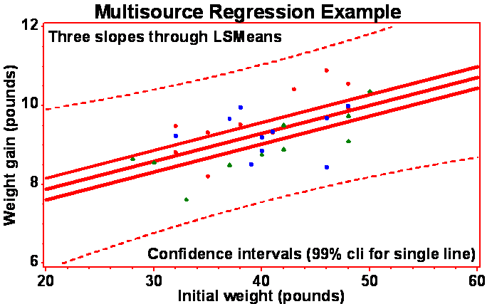
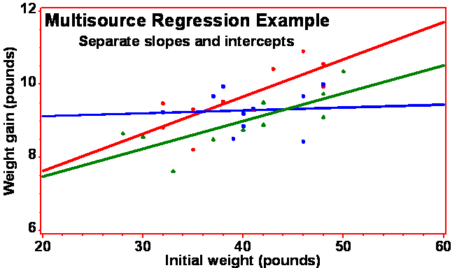
TITLE1 F=SWISS H=1 'Multisource Regression Example';
1949
TITLE2 F=SWISS H=1 'Separate slopes and intercepts';
1950
PLOT
A*X B*X C*X / OVERLAY HAXIS=AXIS1 VAXIS=AXIS2;
1951
AXIS1
LABEL=(F=SWISS H=1 'Initial weight (pounds)') WIDTH=5 MINOR=(N=4)
1952
VALUE=(F=SWISS H=1) ORDER=0 TO 60 BY 10;
1953
AXIS2
LABEL=(F=SWISS H=1 'Weight gain (pounds)') WIDTH=6
1954
VALUE=(F=SWISS H=1) MINOR=(N=5) ORDER=6 TO 12 BY 2;
1955
SYMBOL1 C=red V=J I=RL L=1 W=2 H=1 F=SPECIAL
MODE=INCLUDE;
1956
SYMBOL2 C=blue V=K I=RL L=1 W=2 H=1 F=SPECIAL MODE=INCLUDE;
1957
SYMBOL3 C=green V=L I=RL L=1 W=2
H=1 F=SPECIAL MODE=INCLUDE; RUN;
WARNING: The
axis frame outline was drawn with line width
6 as specified on the left vertical axis. Any other axis line widths
were
ignored.
NOTE:
Regression equation : A =
5.598712 + 0.101766*X.
NOTE: 20
observation(s) contained a MISSING value for the
A * X request.
NOTE:
Regression equation : B =
8.969529 + 0.007825*X.
NOTE: 20
observation(s) contained a MISSING value for the
B * X request.
NOTE:
Regression equation : C =
5.953836 + 0.075934*X.
NOTE: 20
observation(s) contained a MISSING value for the
C * X request.

NOTE: 26
RECORDS
WRITTEN TO
C:\Geaghan\EXST\EXST7015New\Fall2002\SAS\25s-AnCova&Design1.cgm
Which
treatment is "higher"?
Where would you compare the lines?
1959
GOPTIONS
GSFNAME=OUT2; FILENAME OUT2
'C:\Geaghan\EXST\EXST7015New\Fall2002\SAS\25s-AnCova&Design2.cgm';
NOTE: There
were 30 observations read from the data set
WORK.TWO.
NOTE:
PROCEDURE GPLOT used:
real
time 0.19
seconds
cpu
time
0.12 seconds
1960
PROC
GPLOT DATA=TWO;
1961
TITLE1 F=SWISS H=1 'Multisource Regression Example';
1962
TITLE2 F=SWISS H=1 'Single line with confidence intervals (99% cli)';
1963
PLOT
Y*X / OVERLAY HAXIS=AXIS1 VAXIS=AXIS2;
1964
AXIS1
LABEL=(F=SWISS H=1 'Initial weight (pounds)') WIDTH=5 MINOR=(N=4)
1965
VALUE=(F=SWISS H=1) ORDER=0 TO 60 BY 10;
1966
AXIS2
LABEL=(F=SWISS H=1 'Weight gain (pounds)') WIDTH=6
1967
VALUE=(F=SWISS H=1) MINOR=(N=5) ORDER=6 TO 12 BY 2;
1968
SYMBOL1 C=red V=J I=RLcli99 L=1 W=2 F=SPECIAL H=1 MODE=INCLUDE;
1969
RUN;
WARNING: The
axis frame outline was drawn with line width
6 as specified on the left vertical axis. Any other axis line widths
were
ignored.
NOTE:
Regression equation : Y =
6.464854 + 0.07081*X.
NOTE: 94
RECORDS
WRITTEN TO
C:\Geaghan\EXST\EXST7015New\Fall2002\SAS\25s-AnCova&Design1.cgm
1970
NOTE: There
were 30 observations read from the data set
WORK.TWO.
NOTE:
PROCEDURE GPLOT used:
real
time 0.11
seconds
cpu
time
0.05 seconds

Modified: August 16, 2004
James P. Geaghan
