Original Program from program editor.
**********************************************************************;
*** EXST7005 Regression Example ***;
*** Redfin Pickerel, and other fish, accumulate parasites ***;
*** on their fins. These parasites attach and stay with ***;
*** the fish throughout its life until the fish is eaten ***;
*** and the parasite continues its life cycle. ***;
*** - - - - - - - - - - - - - - - - - - - - - - - - - - - - - - - -***;
*** If parasites are accumulated at a constant rate, older ***;
*** fish should have more parasites. Test this hypothesis. ***;
*** OBJECTIVES: ***;
*** 1) Determine if older fish have more parasites. ***;
*** 2) Estimate the rate of accumulation of parasites. ***;
*** 3) Place a confidence interval on this estimate ***;
*** 4) Estimate the intercept with confidence interval. ***;
*** 5) Determine how many parasites a 10 year old fish would have. ***;
*** 6) Place a confidence interval on the 10 year old fish estimate***;
*** 7) Determine of a linear model is adequate. ***;
*** 8) An old published article states that the rate of accumul. ***;
*** should be about 5 per year. Test our estimate against 5. ***;
**********************************************************************;
options ps=256 ls=99 nocenter nodate nonumber nolabel;
TITLE1 'Example of Simple linear Regression (SLR)';
DATA ONE; INFILE CARDS MISSOVER;
TITLE2 'Rate of parasite accumulation in Redfin Pickerel';
INPUT AGE PARASITE;
LABEL AGE = 'Fish age from scales reading';
LABEL PARASITE = 'Pectoral fin parasites / sq cm';
CARDS;
1 3
2 7
3 8
3 12
3 10
4 15
4 14
5 16
6 17
6 15
6 16
7 19
7 21
8 18
9 17
9 20
0 .
10 .
;
PROC PRINT DATA=ONE;
TITLE3 'Data Listing for Fish Parasite Regression'; RUN;
PROC REG DATA=ONE LINEPRINTER;
TITLE3 'Fish Parasite example using REG with CLM';
MODEL PARASITE=AGE / clb; *** CLI CLM P R; ID AGE;
TEST AGE=5;
OUTPUT OUT=NEXT P=P R=E STUDENT=student rstudent=rstudent
lcl=lcl lclm=lclm ucl=ucl uclm=uclm;
RUN; OPTIONS PS=35; TITLE4 'Plots of raw data & residuals';
PLOT PREDICTED.*AGE='P' PARASITE*AGE='O' / OVERLAY;
PLOT RESIDUAL.*AGE='E';
RUN; QUIT;
proc print data=next;
TITLE4 'Listing of output from PROC REG';
var age parasite P E student rstudent lcl lclm ucl uclm; run;
OPTIONS PS=61;
PROC UNIVARIATE DATA=NEXT NORMAL PLOT; VAR E;
TITLE4 'Residual analysis with PROC UNIVARIATE';
RUN;
PROC GLM DATA=ONE;
TITLE3 'Fish Parasite example using GLM with CLI';
MODEL PARASITE=AGE / P CLI ALPHA=.01; ID AGE;
CONTRAST 'HO: B1 = 5' AGE 5;
RUN; QUIT;
GGOPTIONS DEVICE=CGMflwa GSFMODE=REPLACE GSFNAME=OUT NOPROMPT noROTATE
ftext='TimesRoman' ftitle='TimesRoman';
FILENAME OUT1 'F:\Fall2003\_Disk_Fall03\slrci2.cgm';
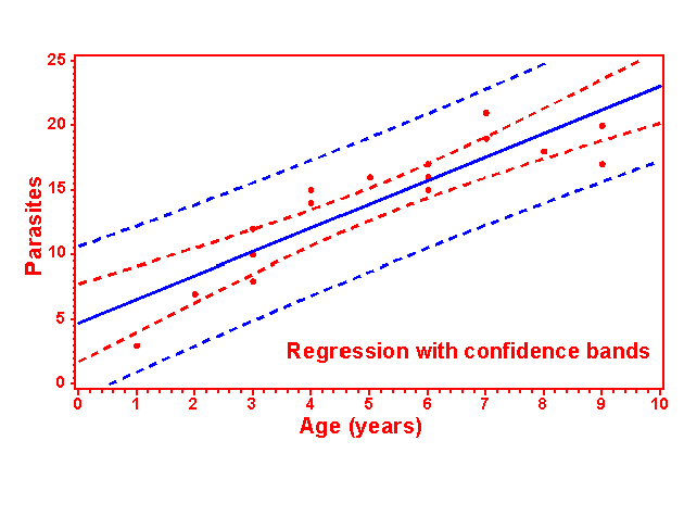
PROC GPLOT DATA=one; TITLE1 'Regression with confidence bands';
PLOT parasite*age=1 parasite*age=2 / OVERLAY HAXIS=AXIS1 VAXIS=AXIS2;
AXIS1 LABEL=('Age (years)') ORDER=0 TO 10 BY 1;
AXIS2 LABEL=('Parasites') ORDER=0 TO 25 BY 5;
SYMBOL1 V=dot c=red I=RLclm95 L=1 W=5 mode=include;
SYMBOL2 V=none c=blue I=RLcli95 L=1 W=5 mode=include; run;
GOPTIONS GSFNAME=OUT2;
FILENAME OUT2 'F:\Fall2003\_Disk_Fall03\resplot2.cgm';
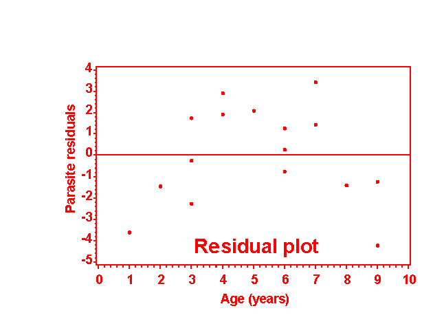
PROC GPLOT DATA=next;
TITLE1 'Residual plot';
PLOT e*age / HAXIS=AXIS1 VAXIS=AXIS2 vref=0;
AXIS1 LABEL=('Age (years)') ORDER=0 TO 10 BY 1;
AXIS2 LABEL=('Parasite residuals');
SYMBOL1 V=dot c=red I=none L=1 W=5 mode=include; run;
quit;
Below is output from the SAS log (bold) and output from the SAS
Output window.
1 **********************************************************************;
2 *** EXST7005 Regression Example ***;
3 *** Redfin Pickerel, and other fish, accumulate parasites ***;
4 *** on their fins. These parasites attach and stay with ***;
5 *** the fish throughout its life until the fish is eaten ***;
6 *** and the parasite continues its life cycle. ***;
7 *** - - - - - - - - - - - - - - - - - - - - - - - - - - - - - - - -***;
8 *** If parasites are accumulated at a constant rate, older ***;
9 *** fish should have more parasites. Test this hypothesis. ***;
10 *** OBJECTIVES: ***;
11 *** 1) Determine if older fish have more parasites. ***;
12 *** 2) Estimate the rate of accumulation of parasites. ***;
13 *** 3) Place a confidence interval on this estimate ***;
14 *** 4) Estimate the intercept with confidence interval. ***;
15 *** 5) Determine how many parasites a 10 year old fish would have. ***;
16 *** 6) Place a confidence interval on the 10 year old fish estimate***;
17 *** 7) Determine of a linear model is adequate. ***;
18 *** 8) An old published article states that the rate of accumul. ***;
19 *** should be about 5 per year. Test our estimate against 5. ***;
20 **********************************************************************;
21
22 options ps=256 ls=99 nocenter nodate nonumber nolabel;
23 TITLE1 'Example of Simple linear Regression (SLR)';
24
25 DATA ONE; INFILE CARDS MISSOVER;
26 TITLE2 'Rate of parasite accumulation in Redfin Pickerel';
27 INPUT AGE PARASITE;
28 LABEL AGE = 'Fish age from scales reading';
29 LABEL PARASITE = 'Pectoral fin parasites / sq cm';
30 CARDS;
NOTE: The data set WORK.ONE has 18 observations and 2 variables.
NOTE: DATA statement used (Total process time):
real time 0.03 seconds
cpu time 0.03 seconds
49 ;
50 PROC PRINT DATA=ONE;
51 TITLE3 'Data Listing for Fish Parasite Regression'; RUN;
NOTE: There were 18 observations read from the data set WORK.ONE.
NOTE: The PROCEDURE PRINT printed page 1.
NOTE: PROCEDURE PRINT used (Total process time):
real time 0.00 seconds
cpu time 0.00 seconds
Example of Simple linear Regression (SLR)
Rate of parasite accumulation in Redfin Pickerel
Data Listing for Fish Parasite Regression
Obs AGE PARASITE
1 1 3
2 2 7
3 3 8
4 3 12
5 3 10
6 4 15
7 4 14
8 5 16
9 6 17
10 6 15
11 6 16
12 7 19
13 7 21
14 8 18
15 9 17
16 9 20
17 0 .
18 10 .
52
53 PROC REG DATA=ONE LINEPRINTER;
54 TITLE3 'Fish Parasite example using REG with CLM';
55 MODEL PARASITE=AGE / clb; *** CLI CLM P R; ID AGE;
56 TEST AGE=5;
57 OUTPUT OUT=NEXT P=P R=E STUDENT=student rstudent=rstudent
58 lcl=lcl lclm=lclm ucl=ucl uclm=uclm;
59 RUN;
NOTE: 18 observations read.
NOTE: 2 observations have missing values.
NOTE: 16 observations used in computations.
59 ! OPTIONS PS=35; TITLE4 'Plots of raw data & residuals';
60 PLOT PREDICTED.*AGE='P' PARASITE*AGE='O' / OVERLAY;
61 PLOT RESIDUAL.*AGE='E';
62 RUN;
62 ! QUIT;
NOTE: The data set WORK.NEXT has 18 observations and 10 variables.
NOTE: The PROCEDURE REG printed pages 2-5.
NOTE: PROCEDURE REG used (Total process time):
real time 0.04 seconds
cpu time 0.04 seconds
Example of Simple linear Regression (SLR)
Rate of parasite accumulation in Redfin Pickerel
Fish Parasite example using REG with CLM
The REG Procedure
Model: MODEL1
Dependent Variable: PARASITE
Analysis of Variance
Sum of Mean
Source DF Squares Square F Value Pr > F
Model 1 301.94955 301.94955 54.86 <.0001
Error 14 77.05045 5.50360
Corrected Total 15 379.00000
Root MSE 2.34598 R-Square 0.7967
Dependent Mean 14.25000 Adj R-Sq 0.7822
Coeff Var 16.46299
Parameter Estimates
Parameter Standard
Variable DF Estimate Error t Value Pr > |t| 95%Confidence Limits
Intercept 1 4.77125 1.40769 3.39 0.0044 1.75205 7.79045
AGE 1 1.82723 0.24669 7.41 <.0001 1.29813 2.35632
The REG Procedure
Model: MODEL1
Test 1 Results for Dependent Variable PARASITE
Mean
Source DF Square F Value Pr > F
Numerator 1 910.38705 165.42 <.0001
Denominator 14 5.50360
�Example of Simple linear Regression (SLR)
Rate of parasite accumulation in Redfin Pickerel
Fish Parasite example using REG with CLM
Plots of raw data & residuals
The REG Procedure
Model: MODEL1
Dependent Variable: PARASITE
-----+----+----+----+----+----+----+----+----+----+----+----+----+----+----+----+----+------
P 30 + +
r | |
e | |
d | |
i | |
c | O P |
t 20 + P O +
e | ? O |
d | O O O |
PRED | O ? |
V | O P |
a | O P |
l 10 + ? +
u | P O |
e | P O |
| |
o | O |
f | |
0 + +
P -----+----+----+----+----+----+----+----+----+----+----+----+----+----+----+----+----+------
A 1.0 1.5 2.0 2.5 3.0 3.5 4.0 4.5 5.0 5.5 6.0 6.5 7.0 7.5 8.0 8.5 9.0
R AGE
The REG Procedure
Model: MODEL1
Dependent Variable: PARASITE
---+----+----+----+----+----+----+----+----+----+----+----+----+----+----+----+----+----
RESIDUAL | |
5.0 + +
| |
| E |
| E |
R 2.5 + +
e | E E E |
s | E E |
i | |
d 0.0 + E E +
u | E |
a | E E E |
l | |
-2.5 + E +
| |
| E |
| E |
-5.0 + +
| |
---+----+----+----+----+----+----+----+----+----+----+----+----+----+----+----+----+----
1.0 1.5 2.0 2.5 3.0 3.5 4.0 4.5 5.0 5.5 6.0 6.5 7.0 7.5 8.0 8.5 9.0
AGE
63 proc print data=next;
64 TITLE4 'Listing of output from PROC REG';
65 var age parasite P E student rstudent lcl lclm ucl uclm; run;
NOTE: There were 18 observations read from the data set WORK.NEXT.
NOTE: The PROCEDURE PRINT printed page 6.
NOTE: PROCEDURE PRINT used (Total process time):
real time 0.01 seconds
cpu time 0.01 seconds
Example of Simple linear Regression (SLR)
Rate of parasite accumulation in Redfin Pickerel
Fish Parasite example using REG with CLM
Listing of output from PROC REG
Obs AGE PARASITE P E student rstudent lcl lclm ucl uclm
1 1 3 6.5985 -3.59848 -1.77879 -1.94833 0.9586 4.0507 12.2384 9.1463
2 2 7 8.4257 -1.42571 -0.66902 -0.65524 2.9719 6.3218 13.8795 10.5296
3 3 8 10.2529 -2.25294 -1.02107 -1.02274 4.9389 8.5436 15.5670 11.9623
4 3 12 10.2529 1.74706 0.79180 0.78068 4.9389 8.5436 15.5670 11.9623
5 3 10 10.2529 -0.25294 -0.11464 -0.11052 4.9389 8.5436 15.5670 11.9623
6 4 15 12.0802 2.91983 1.29626 1.33156 6.8558 10.6741 17.3046 13.4863
7 4 14 12.0802 1.91983 0.85231 0.84348 6.8558 10.6741 17.3046 13.4863
8 5 16 13.9074 2.09261 0.92144 0.91614 8.7200 12.6456 19.0948 15.1692
9 6 17 15.7346 1.26538 0.55925 0.54503 10.5304 14.4053 20.9389 17.0640
10 6 15 15.7346 -0.73462 -0.32468 -0.31405 10.5304 14.4053 20.9389 17.0640
11 6 16 15.7346 0.26538 0.11729 0.11308 10.5304 14.4053 20.9389 17.0640
12 7 19 17.5619 1.43815 0.64577 0.63176 12.2875 15.9801 22.8362 19.1436
13 7 21 17.5619 3.43815 1.54382 1.63316 12.2875 15.9801 22.8362 19.1436
14 8 18 19.3891 -1.38908 -0.64222 -0.62818 13.9934 17.4406 24.7848 21.3376
15 9 17 21.2163 -4.21631 -2.03920 -2.34368 15.6514 18.8391 26.7812 23.5936
16 9 20 21.2163 -1.21631 -0.58826 -0.57400 15.6514 18.8391 26.7812 23.5936
17 0 . 4.7713 . . . -1.0967 1.7520 10.6392 7.7905
18 10 . 23.0435 . . . 17.2657 20.2035 28.8213 25.8836
66 OPTIONS PS=61;
67 PROC UNIVARIATE DATA=NEXT NORMAL PLOT; VAR E;
68 TITLE4 'Residual analysis with PROC UNIVARIATE';
69 RUN;
NOTE: The PROCEDURE UNIVARIATE printed pages 7-9.
NOTE: PROCEDURE UNIVARIATE used (Total process time):
real time 0.01 seconds
cpu time 0.01 seconds
Example of Simple linear Regression (SLR)
Rate of parasite accumulation in Redfin Pickerel
Fish Parasite example using REG with CLM
Residual analysis with PROC UNIVARIATE
The UNIVARIATE Procedure
Variable: E
Moments
N 16 Sum Weights 16
Mean 0 Sum Observations 0
Std Deviation 2.26642816 Variance 5.13669661
Skewness -0.3183952 Kurtosis -0.7591259
Uncorrected SS 77.0504492 Corrected SS 77.0504492
Coeff Variation . Std Error Mean 0.56660704
Basic Statistical Measures
Location Variability
Mean 0.000000 Std Deviation 2.26643
Median 0.006220 Variance 5.13670
Mode . Range 7.65446
Interquartile Range 3.24084
Tests for Location: Mu0=0n
Test -Statistic- -----p Value------
Student's t t 0 Pr > |t| 1.0000
Sign M 0 Pr >= |M| 1.0000
Signed Rank S 4 Pr >= |S| 0.8603
Tests for Normality
Test --Statistic--- -----p Value------
Shapiro-Wilk W 0.961962 Pr < W 0.6975
Kolmogorov-Smirnov D 0.149185 Pr > D >0.1500
Cramer-von Mises W-Sq 0.038869 Pr > W-Sq >0.2500
Anderson-Darling A-Sq 0.248615 Pr > A-Sq >0.2500
Quantiles (Definition 5)
Quantile Estimate
100% Max 3.43814789
99% 3.43814789
95% 3.43814789
90% 2.91983414
75% Q3 1.83344851
50% Median 0.00621977
25% Q1 -1.40739461
10% -3.59847961
5% -4.21630961
1% -4.21630961
Quantiles (Definition 5)
Quantile Estimate
0% Min -4.21630961
Extreme Observations
------Lowest----- -----Highest-----
Value Obs Value Obs
-4.21631 15 1.74706 4
-3.59848 1 1.91983 7
-2.25294 3 2.09261 8
-1.42571 2 2.91983 6
-1.38908 14 3.43815 13
Missing Values -----Percent Of-----
Missing Missing
Value Count All Obs Obs
. 2 11.11 100.00
Stem Leaf Boxplot
3 4 1 |
2 19 2 |
1 3479 4 +-----+
0 3 1 *--+--*
-0 73 2 | |
-1 442 3 +-----+
-2 3 1 |
-3 6 1 |
-4 2 1 |
----+----+----+----+
The UNIVARIATE Procedure
Variable: E
Normal Probability Plot
3.5+ ++++*
| +*++*
| * *+*+*
| +*+++
-0.5+ ++**
| *+*+*
| +++*+
| ++++*
-4.5+ ++++*
+----+----+----+----+----+----+----+----+----+----+
-2 -1 0 +1 +2
71 PROC GLM DATA=ONE;
72 TITLE3 'Fish Parasite example using GLM with CLI';
73 MODEL PARASITE=AGE / P CLI ALPHA=.01; ID AGE;
74 CONTRAST 'HO: B1 = 5' AGE 5;
75 RUN;
75 ! QUIT;
NOTE: The PROCEDURE GLM printed pages 10-13.
NOTE: PROCEDURE GLM used (Total process time):
real time 0.03 seconds
cpu time 0.03 seconds
Example of Simple linear Regression (SLR)
Rate of parasite accumulation in Redfin Pickerel
Fish Parasite example using GLM with CLI
The GLM Procedure
Number of observations 18
NOTE: Due to missing values, only 16 observations can be used in this analysis.
Dependent Variable: PARASITE
Sum of
Source DF Squares Mean Square F Value Pr > F
Model 1 301.9495508 301.9495508 54.86 <.0001
Error 14 77.0504492 5.5036035
Corrected Total 15 379.0000000
R-Square Coeff Var Root MSE PARASITE Mean
0.796701 16.46299 2.345976 14.25000
Source DF Type I SS Mean Square F Value Pr > F
AGE 1 301.9495508 301.9495508 54.86 <.0001
Source DF Type III SS Mean Square F Value Pr > F
AGE 1 301.9495508 301.9495508 54.86 <.0001
Contrast DF Contrast SS Mean Square F Value Pr > F
HO: B1 = 5 1 301.9495508 301.9495508 54.86 <.0001
� Standard
Parameter Estimate Error t Value Pr > |t|
Intercept 4.771250864 1.40769370 3.39 0.0044
AGE 1.827228749 0.24668872 7.41 <.0001
Observation AGE Observed Predicted Residual
1 1 3.00000000 6.59847961 -3.59847961
2 2 7.00000000 8.42570836 -1.42570836
3 3 8.00000000 10.25293711 -2.25293711
4 3 12.00000000 10.25293711 1.74706289
5 3 10.00000000 10.25293711 -0.25293711
6 4 15.00000000 12.08016586 2.91983414
7 4 14.00000000 12.08016586 1.91983414
8 5 16.00000000 13.90739461 2.09260539
9 6 17.00000000 15.73462336 1.26537664
10 6 15.00000000 15.73462336 -0.73462336
11 6 16.00000000 15.73462336 0.26537664
12 7 19.00000000 17.56185211 1.43814789
13 7 21.00000000 17.56185211 3.43814789
14 8 18.00000000 19.38908086 -1.38908086
15 9 17.00000000 21.21630961 -4.21630961
16 9 20.00000000 21.21630961 -1.21630961
17 * 0 . 4.77125086 .
18 * 10 . 23.04353836 .
99%Confidence Limits for
Observation AGE Individual Predicted Value
1 1 -1.22936390 14.42632313
2 2 0.85616543 15.99525129
3 3 2.87734381 17.62853041
4 3 2.87734381 17.62853041
5 3 2.87734381 17.62853041
6 4 4.82900575 19.33132597
7 4 4.82900575 19.33132597
8 5 6.70754602 21.10724320
9 6 8.51140616 22.95784055
10 6 8.51140616 22.95784055
11 6 8.51140616 22.95784055
12 7 10.24130132 24.88240289
13 7 10.24130132 24.88240289
14 8 11.90011489 26.87804682
15 9 13.49249521 28.94012400
16 9 13.49249521 28.94012400
17 * 0 -3.37312377 12.91562550
18 * 10 15.02427676 31.06279995
* Observation was not used in this analysis
Example of Simple linear Regression (SLR)
Rate of parasite accumulation in Redfin Pickerel
Fish Parasite example using GLM with CLI
The GLM Procedure
Sum of Residuals -0.0000000
Sum of Squared Residuals 77.0504492
Sum of Squared Residuals - Error SS -0.0000000
PRESS Statistic 110.4690933
First Order Autocorrelation 0.3362460
Durbin-Watson D 1.1402481
77 GOPTIONS DEVICE=CGMflwa GSFMODE=REPLACE GSFNAME=OUT NOPROMPT noROTATE
78 ftext='TimesRoman' ftitle='TimesRoman';
79
80 FILENAME OUT1 'F:\Fall2003\_Disk_Fall03\slrci2.cgm';
81 PROC GPLOT DATA=one; TITLE1 'Regression with confidence bands';
82 PLOT parasite*age=1 parasite*age=2 / OVERLAY HAXIS=AXIS1 VAXIS=AXIS2;
83 AXIS1 LABEL=('Age (years)') ORDER=0 TO 10 BY 1;
84 AXIS2 LABEL=('Parasites') ORDER=0 TO 25 BY 5;
85 SYMBOL1 V=dot c=red I=RLclm95 L=1 W=5 mode=include;
86 SYMBOL2 V=none c=blue I=RLcli95 L=1 W=5 mode=include; run;
NOTE: Regression equation : PARASITE = 4.771251 + 1.827229*AGE.
NOTE: 2 observation(s) contained a MISSING value for the PARASITE * AGE request.
NOTE: Regression equation : PARASITE = 4.771251 + 1.827229*AGE.
NOTE: 2 observation(s) contained a MISSING value for the PARASITE * AGE request.
WARNING: GSFNAME OUT has not been assigned.
NOTE: GSFNAME OUT temporarily assigned to F:\Fall2003\_Disk_Fall03\sasgraph.cgm.
NOTE: 82 RECORDS WRITTEN TO F:\Fall2003\_Disk_Fall03\sasgraph.cgm
87
88
89 GOPTIONS GSFNAME=OUT2;
90 FILENAME OUT2 'F:\Fall2003\_Disk_Fall03\resplot2.cgm';
NOTE: There were 18 observations read from the data set WORK.ONE.
NOTE: PROCEDURE GPLOT used:
real time 0.93 seconds
91 PROC GPLOT DATA=next;
92 TITLE1 'Residual plot';
93 PLOT e*age / HAXIS=AXIS1 VAXIS=AXIS2 vref=0;
94 AXIS1 LABEL=('Age (years)') ORDER=0 TO 10 BY 1;
95 AXIS2 LABEL=('Parasite residuals');
96 SYMBOL1 V=dot c=red I=none L=1 W=5 mode=include; run;
NOTE: 2 observation(s) contained a MISSING value for the E * AGE request.
NOTE: 21 RECORDS WRITTEN TO F:\Fall2003\_Disk_Fall03\resplot2.cgm
97 quit;
NOTE: There were 18 observations read from the data set WORK.NEXT.
NOTE: PROCEDURE GPLOT used:
real time 0.16 seconds
Last modified
by James P. Geaghan
on Wednesday, August 13, 2003