EXST SAS Lab

Lab 10: Analysis of Variance

---

Objectives

1. Input a CSV file and examine the data with a boxplot

2. Do an Analysis of Variance (ANOVA) in PROC MIXED. Include:

· Output of residuals PROC MIXED

· LSMeans with a Tukey adjustment

· ODS output for a macro called PDMix800.sas

3. Run PDMIX800.sas macro

4. Use PROC UNIVARIATE to test the residuals for normality

5. Run a second ANOVA with PROC MIXED,
exactly like the first, but with a test of homogeneity of variance

This week’s assignment includes the use of a MACRO. The macro, “pdmix800.sas”, is linked to the lab assignment page. You need to download the program and put it in the “current folder”, or in a known directory like “C:\TEMP”. You do not need to include this SAS program as part of your SAS program. You only need to put an “%include” statement in your program to indicate where the macro can be found. Your program will then be able to access the macro just as if it was part of your program.

The example

The datasets for this example and assignment were drawn from Chapter 6 of your textbook (Freund, Rudolph J., William J. Wilson and Donna L. Mohr. 2010. Statistical Methods. Academic Press (ELSIVIER), N.Y.). The example data set is a CSV file. (Exercise 6.11, Table 6.37). It is a true “multivariable” data set, though it only has two variables in addition to the group, or categorical, variable. However, only one of the two variables is to be analyzed so no special output is required. The data set for the assignment only has a single variable in addition to the categorical variable.

The description of the data set in the text is as follows.

“Serious environmental problems arise from absorption into soil of metals that escape into the air from different industrial operations. To ascertain if absorption rates differ among soil types, six soil samples were randomly selected from fields having five different soil types (A, B, C, D, and E) in an area known to have relatively uniform exposure to the metals studied. The 30 soil samples were analyzed for cadmium (Cd) and lead (Pb) content. Data for the two metals are to be analyzed separately.”

After the usual heading information, the input statements were:

title1 "Assignment 09 - Cadmium content in soil example";

data MetalContent;

INFILE 'datatab_6_37.csv' dlm=',' dsd missover firstobs=2;

input soil $ Cadmium Lead;

datalines;

;

run;

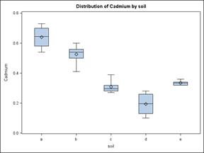
First a box plot is used to examine the data more closely. Does it appear as though there are likely to be differences in means? Is the data symmetric? Are the variances homogeneous?

PROC BOXPLOT data=MetalContent;

plot Cadmium*soil; run;

From the box plot, the means look to be quite different. It also appears that the data is reasonably symmetric, so possibly normal, and that the variances may not be equal to each other (i.e. homogenous). These assumptions will have to be checked.

Each line in the MIXED procedure below is labeled in order to discuss the function of each line individually. 

a	PROC MIXED data=MetalContent cl covtest;
b	TITLE2 'Analysis of Variance using PROC MIXED';
c	class soil;
d	model Cadmium = soil / outp=outputstuff;
e	lsmeans soil / adjust=tukey cl;
f	ods output diffs=ppp lsmeans=mmm;
g	*ods exclude diffs lsmeans;
h	run;
i	%include 'pdmix800.sas';
j	%pdmix800(ppp,mmm,alpha=0.05,sort=yes);
k	RUN;

Line “a” starts the procedure (mixed) to be run on a dataset called METALCONTENT. I have added the options cl and covtest which provide confidence interval and a test on the random components (e.g. H₀: s² = 0). The only random component in this model will be the residual error term from the pooled within group deviations. We have seen title and class statements before (lines “b” and “c”), and they work the same way here as elsewhere.

Line “d”, the model statement, represents the linear model for the one-way ANOVA, Y_ij = m + t_i + e_ij, , where Y_ij is the variable to be analyzed (cadmium), m represents the mean (correction factor or correction for the mean), t_i represents the effect of treatment “i” (soil), and e_ij represents the within group deviations, or residuals. In the SAS model statement the correction factor (m) is assumed, and fitted by default, and e_ij automatically becomes the residual error term. So, for a one-way ANOVA only the treatment variable name need occur in the model. For models with several error terms the residual is the one at the lowest level in the hierarchy and others would be listed in a random statement. A random statement is not needed for this example.

Any options that are desired for the model statement are placed after the slash, “/”. In this case the only option is the OUTP=SomeDataSetName which will produce a new dataset that will include all the variables of the original dataset (metalcontent) plus some new variables created by PROC MIXED, notably the residuals in a variable called resid and the predicted values in a variable called pred.

When the variances are unequal, ANOVA has the same unknown degrees of freedom issues as the two sample t-test. proc mixed can fit and work with unequal variances. In that case you may specify the ddfm= option. DDFM is denominator degree of freedom method. Although the Satterthwaite approximation method is available (DDFM=Sat), a more recently developed option, the Kenward-Rogers approximation (DDFM=KR), is probably a better option. Other options for DDFM are available and there are other options for the model statement in addition to OUTP= and DDFM=.

There are two sections of the analysis of variance done with proc mixed that may be of particular interest. The first is the “Covariance Parameter Estimates” section. This section gives the value of the residual and any other random components to the model. Also provided, if requested, is a Z-test of the estimate against zero and a confidence interval.

Covariance Parameter Estimates

                         Standard      Z

Cov Parm    Estimate      Error  Value Pr > Z  Alpha      Lower     Upper

Residual    0.003325  0.000940   3.54    0.0002   0.05  0.002045  0.006335

The key element of the PROC MIXED is the test of treatment means (). This is usually the primary objective of the analysis.

Type 3 Tests of Fixed Effects

Num     Den

Effect         DF      DF    F Value    Pr > F

soil            4      25      58.00    <.0001

In this case there appears to be a highly significant difference among the treatment means. The next objective is to determine how the treatment means differ from each other.

Line “e” produces the LSMeans, estimates for each of the levels of the variable listed. The line “lsmeans soil / adjust=tukey cl;” will produce means for the SOIL variable and the “cl” option requests confidence intervals be listed for the estimated soil means. The Least Square Means output below gives the least squares estimate, the standard error of the estimate, a t-test of the estimate against zero and the 95% confidence interval of the estimate. The t-test of the estimate against zero is not usually a useful test. In Analysis of Variance the objective is to test the means against each other, not individually against zero.

Least Squares Means

                       Standard

Effect soil  Estimate     Error    DF  t Value  Pr > |t|  Alpha    Lower    Upper

soil    a      0.6400   0.02354    25    27.19    <.0001   0.05   0.5915   0.6885

soil    b      0.5250   0.02354    25    22.30    <.0001   0.05   0.4765   0.5735

soil    c      0.3083   0.02354    25    13.10    <.0001   0.05   0.2599   0.3568

soil    d      0.1933   0.02354    25     8.21    <.0001   0.05   0.1449   0.2418

soil    e      0.3350   0.02354    25    14.23    <.0001   0.05   0.2865   0.3835

The LSMEANS statement will also produce pairwise comparisons of each soil level against all the others. These comparisons will be produced both with and without the requested TUKEY adjustment (discussed in class). The comparison below for soil “a” versus soil “b” shows a P value for the pairwise LSD of 0.0020 and a Tukey adjusted pairwise test value of 0.0155. Confidence intervals have not been included with the output below.

Differences of Least Squares Means

                               Standard

Effect soil _soil    Estimate     Error    DF  t Value  Pr > |t|   Adjustment      Adj P

soil    a     b        0.1150   0.03329    25     3.45    0.0020        Tukey     0.0155

soil    a     c        0.3317   0.03329    25     9.96    <.0001        Tukey     <.0001

soil    a     d        0.4467   0.03329    25    13.42    <.0001        Tukey     <.0001

soil    a     e        0.3050   0.03329    25     9.16    <.0001        Tukey     <.0001

soil    b     c        0.2167   0.03329    25     6.51    <.0001        Tukey     <.0001

soil    b     d        0.3317   0.03329    25     9.96    <.0001        Tukey     <.0001

soil    b     e        0.1900   0.03329    25     5.71    <.0001        Tukey     <.0001

soil    c     d        0.1150   0.03329    25     3.45    0.0020        Tukey     0.0155

soil    c     e      -0.02667   0.03329    25    -0.80    0.4307        Tukey     0.9278

soil    d     e       -0.1417   0.03329    25    -4.26    0.0003        Tukey     0.0022

A note on post hoc tests

The primary tool for assessing statistical significance in analysis of variance is the overall test of treatments; always start with this. If this test is not significant, you are done unless there are some a priori hypotheses. In the event that the null hypothesis of equal treatment means is rejected (i.e. P-value < a), interpretation may be facilitated with contrasts or some post hoc assessment tools. SAS will do a number of different post hoc adjustments for comparing the means of the different treatment levels. Each has a different objective, so only one is appropriate and proper for a particular case.

A statistical pairwise hypothesis test, or comparison, (e.g.) has a probability of Type I error equal to a. We refer to this as a comparison-wise error rate. When many comparisons are done, the error rate for the experiment increases with each additional test. This is the experiment-wise error rate. The intent of the post hoc adjustments is to maintain an overall experiment-wise error rate of a for more than one comparison. The more traditional adjustments are as follows.

LSD	This is the default and no adjustment is made to the error rate. Every comparison has a probability of error equal to alpha. This is a comparison-wise error rate, and it is included on every test of LSMeans differences in addition to any other adjustments requested.
DUNNETT	An adjustment intended to maintain an overall error rate of alpha for comparing one level of a treatment (e.g. a control) pairwise with all the other treatment levels. This adjustment can be done as a one-tailed test. This is an experiment-wise error rate for this subset of comparisons.
TUKEY	This adjustment is intended to maintain an overall error rate of alpha for comparing all pairwise tests. That is, every mean is compared to every other mean. This is an experiment-wise error rate for this subset of comparisons.
SCHEFFE	This adjustment intended to maintain an overall error rate of alpha for every possible comparison. This includes not only all pairwise tests but also comparisons of subgroups of means to other means or subgroups. This is an experiment-wise error rate for all possible comparisons.
BON	A simple approximation assuming that errors are additive (they aren’t). If “k” tests are to be done each is examined an error rate of alpha / k (i.e. a/k). This is an upper bound of the error rate for this subset of k comparisons.

Note that “alpha” will generally be (a/2) since most of these are two-tailed tests.

The Macro

In the proc mixed program, the 5 lines “f” through “j” were added to run what I refer to as “Saxton’s macro”, PDMIX800.SAS. Within this macro program is an example, and the 5 lines are copied with minimal changes directly from inside the macro. Line “f”, the ODS OUTPUT line, causes two SAS datasets to be created from the LSMEANS statement. The first (mmm) contains the actual lsmeans estimates and the second (ppp) the pairwise comparison P-values. These datasets will be used by the macro. The “g” line would suppress the listing of the lsmeans estimates and the pairwise test of differences since the macro output will give the same information. I often suppress the tests of differences because these can occupy many pages, but I usually like to see the LSMeans estimates. For the assignment I want to see all this output, so I have made this statement a comment.

Line “h” executes the PROC MIXED statement with all the statements and options preceding that line. Line “i” tells your program where your copy of PDMIX800.SAS is stored. If it is in the current folder you only need to give the macro name. Finally, line “j” calls the macro. The example within Saxton’s macro specifies an alpha=0.01, and I usually change this to alpha=0.05. Line “k” runs everything up to this point. The macro will prepare and output the means as a multiple range test with the adjustment specified on the LSMEANS.

The macro conducts a “range test” style of presentation, sorting the means from highest to lowest and indicating those which are significantly different by giving them a separate letter grouping. From the letter groups in the left column below it is clear that the estimate for soil “a” is different from the others because soils “a” is in group A and there are no other members of this group. Soils “b” and “d” are also members of their own group of one. Only group C with soils “e” and “c” are members of the same group indicating that these two soils are not significantly different from each other.

Effect=soil   Method=Tukey(P<0.05)   Set=1

                           Standard                                     Letter

Obs    soil    Estimate       Error     Alpha       Lower       Upper    Group

 1      a        0.6400     0.02354      0.05      0.5915      0.6885       A

 2      b        0.5250     0.02354      0.05      0.4765      0.5735       B

 3      e        0.3350     0.02354      0.05      0.2865      0.3835       C

 4      c        0.3083     0.02354      0.05      0.2599      0.3568       C

 5      d        0.1933     0.02354      0.05      0.1449      0.2418       D

The next output, a proc univariate with a test of normality, is something we have done. The difference here is that we are executing the program on the residuals output from the ANOVA, but the approach, test and interpretation are the same as for the t-tests.

Testing for equal variances among treatments

The PROC MIXED in the example is run a second time. I have removed the lines “e” through “j” and inserted a new line, “repeated / group=soil;”. This new statement will run the GROUP=SOIL option that will test for homogeneity of variance among the specified variable (e.g. soil). This group= option must go on either a REPEATED statement or a RANDOM statement. This analysis doesn’t require either one of these because it has neither repeated nor random components. However, the repeated statement can be used to include the group= option without actually having a repeated variable, so we used it. The random statement cannot be used without an actual random component in the model.

When no group statement is included, as in the first example, homogeneous variance is assumed and the variance is pooled. The group= statement causes PROC MIXED to fit separate variances that can be seen in the “Covariance Parameter Estimates” output section.

Covariance Parameter Estimates

                            Standard       Z

Cov Parm  Group Estimate     Error   Value  Pr > Z  Alpha     Lower     Upper

Residual  soil a  0.005160  0.003263    1.58  0.0569   0.05  0.002011   0.03104

Residual  soil b  0.004390  0.002776    1.58  0.0569   0.05  0.001711   0.02641

Residual  soil c  0.001897  0.001200    1.58  0.0569   0.05  0.000739   0.01141

Residual  soil d  0.004947  0.003129    1.58  0.0569   0.05  0.001927   0.02976

Residual  soil e  0.000230  0.000145    1.58  0.0569   0.05  0.000090  0.001384

Notice that the results of the test of treatment differences has changed. Also note that the standard errors of the estimates in the LSMeans are no longer the same.

Type 3 Tests of Fixed Effects

Num     Den

Effect         DF      DF    F Value    Pr > F

soil            4    8.75      37.16    <.0001

Least Squares Means

                        Standard

Effect  soil  Estimate     Error    DF  t Value  Pr > |t|   Alpha     Lower     Upper

soil    a       0.6400   0.02933     5    21.82    <.0001    0.05    0.5646    0.7154

soil    b       0.5250   0.02705     5    19.41    <.0001    0.05    0.4555    0.5945

soil    c       0.3083   0.01778     5    17.34    <.0001    0.05    0.2626    0.3540

soil    d       0.1933   0.02871     5     6.73    0.0011    0.05    0.1195    0.2671

soil    e       0.3350  0.006191     5    54.11    <.0001    0.05    0.3191    0.3509

Since the variances are no longer homogeneous the pairwise tests of the LSMeans will change. The means are still the same as before. The change is due to the calculation of a variance between the two means with separate variances, , instead of a pooled variance, .

Effect=soil   Method=Tukey-Kramer(P<0.05)   Set=1

Standard Letter

Obs   soil   Estimate       Error    Alpha     Lower     Upper    Group

 1     a       0.6400     0.02933     0.05    0.5646    0.7154      A 

 2     b       0.5250     0.02705     0.05    0.4555    0.5945      A 

 3     e       0.3350    0.006191     0.05    0.3191    0.3509      B 

 4     c       0.3083     0.01778     0.05    0.2626    0.3540      B 

 5     d       0.1933     0.02871     0.05    0.1195    0.2671      C 

There are two ways to determine which model is better, either with pooled variance or with separate variances. When available, the output section “Null Model Likelihood Ratio Test” tests for a difference between a null model with equal variances and the model with separate variances requested by the GROUP= statement. If there is no difference (P-value > a), the simpler, “reduced model” that uses fewer degrees of freedom (e.g. the pooled variance version) is better. However, if there is a statistically significant difference, the fuller model that fits separate variances, each using another degree of freedom, has more information and is the better model. The results of this test for this example indicates that the variances are not homogeneous (P=0.0316).

Null Model Likelihood Ratio Test

   DF    Chi-Square      Pr > ChiSq

    4         10.59          0.0316

The second way of choosing the best model is to examine the “Fit Statistics” output section. The model with the smaller value of the AIC is assumed to be the better model. The very similar AICC or BIC can also be used as a criterion. The AIC value for the full model was -63.3 and for the reduced model was -60.8. As a negative value -63.3 is smaller than -60.8, so the full model is indicated as the better model.

Fit Statistics

-2 Res Log Likelihood           -73.3

AIC (smaller is better)         -63.3

AICC (smaller is better)        -60.2

BIC (smaller is better)         -56.3

This measure does not provide a P-value so it does not indicate if the degree of difference is statistically meaningful.

Assignment 10

The assignment dataset (Exercise 6.12, Table 6.38) comes from a study of growth mediums for fungi. It is a simple dataset with one variable to be analyzed, the diameter of fungal colonies, and a single qualitative (i.e. class) variable for the type of medium used. The description from Freund, Rudolph J., William J. Wilson and D onna L. Mohr. 2010. Statistical Methods. Academic Press (ELSIVIER), N.Y. is as follows:

“For laboratory studies of an organism, it is important to provide a medium in which the organism flourishes. The data for this exercise are from Table 6.38 in you text. The data are from a completely randomized design with four samples for each of seven media. The response is the diameters of the colonies of fungus.”

· Water Agar (WA)

· Cornmeal Agar (CMA)

· Potato Carrot Agar (PCA)

· Potato Dextrose Agar (PDA)

· Tap Water Agar (TWA)

· Rice Dextrose Agar (RDA)

· Nutrient Agar (NA)

Answer all questions about hypothesis tests by stating the outcome (REJECT the null hypothesis or FAIL to reject the null hypothesis) and give a P-value where possible. In particular, the four questions with point value in bold should be answered with a P value.

Turn in your log and the list output or results viewer output. You may write answers to questions either on the log, or on a separate page.

Task 1: Prepare a PROC BOXPLOT for the fungi medium treatments.

Question 1: Does the box plot appear to suggest separate variances or means? ....................  (1 point)

Task 2a: Do an ANOVA using PROC MIXED for the fungi medium treatments. ..........................  (1 point)

2b) include a LSMeans statement with adjust=tukey and cl options. ...........................  (1 point)

2c) include the statements for Saxton’s macro. ....................................................................  (1 point)

Question 2: Are there statistically significant differences among the media treatments? ......  (1 point)

Question 3: What is the P-value (Tukey adjusted) for the two means that are farthest apart? .........  (1 point)

Task 3: Test the residuals from the ANOVA for the assumption of normality.

Question 4: Is the hypothesis of “normality” rejected? ...........  (1 point)

Task 4: Do a second PROC MIXED with a repeated statement in order to test for homogeneity of variance. .............................................................................................................................  (1 point)

Question 5: Do the results indicate that the variances should be pooled for this analysis, or fitted separately? ..........................................................................................................  (1 point)

Question 6: Which model has the smallest AIC (between the model with pooled variance or with variances fitted separately)?  .............................................................................  (1 point)

Save your program for next week. We will do some additional analyses on the same ANOVA.