EXST SAS Lab

Lab #9: Two-sample t-tests

---

Objectives

1. Input a CSV file (data set #1) and do a one-tailed two-sample t-test

2. Input a TXT file (data set #2) and do a two-tailed two-sample t-test

3. Test the two classes in data set #2 for normality and obtain confidence intervals for each

4. Produce BOXPLOTS for the second data set

In this week’s assignment, working from a current folder and naming the HTML output data file are optional; good practices, but optional. Also, you will not have to deal with multiple observations on an input line. The example program does have multiple observations on a line, and two SAS work files will be created from one input file in order to compare the two-sample test to the one-sample test. However, this is not required as part of the assignment program.

Recall that you can get the current folder by opening a SAS file from that directory. If you want to change the directory then double click on the directory (i.e. folder) name on the right side of the bottom bar of the SAS window and you can change it to whatever you want.

The examples

All examples and datasets for this assignment were drawn from Chapter 5 of Freund, Rudolph J. and William J. Wilson. 2003. Statistical Methods, Academic Press, N.Y. The first data set in the example is a CSV file. This file has been used before (Exercise 5.3, Table 5.13) for the paired t-test. It is two areas of a city that were sampled simultaneously and were, therefore, paired. Now they will be analyzed as if they were not sampled simultaneously, but rather as if each area was sampled on different, randomly-selected date. You do not have to do this for the assignment; it is being done just to compare the previous paired t-test result to the two-sample t-test result. In the assignment you will only need to do two-sample t-tests.

The Exercise 5.3 dataset had two separate columns for the two areas in order to calculate a difference for the paired t-test. I also output a second data set with a class (categorical or group) variable in order to do the two-sample t-test. This is from a previous lab exercise.

data Multi (keep=AreaA AreaB diff)

      Pollution (keep=Area index);

   INFILE 'datatab_5_13b.csv' dlm=',' dsd missover firstobs=2;

input AreaA AreaB;

        diff = AreaA - AreaB; output multi;

        Area = 'A'; Index = AreaA; Output Pollution;

        Area = 'B'; Index = AreaB; Output Pollution;

datalines; run;

;

run;

Both tests were done as one-tailed tests with proc ttest as follows. Note that in your assignment you only need to run a t-test test similar to the second one below.

PROC ttest data=multi sides=u;

   title2 'Pollution example done as a paired t-test with Proc TTEST';

   TITLE3 'One-tailed hypothesis';

   VAR diff;

RUN;

PROC ttest data=Pollution sides=u;

   title2 'Pollution example done as a tw0-sample t-test with Proc TTEST';

   TITLE3 'One-tailed hypothesis';

   CLASS area;

   VAR Index;

If you examine the values in the dataset above, it is pretty clear that the data is actually paired. When one area has a high index value, the other area is also relatively high. The two areas tend to go up and down together. The paired t-test (below) should have much less variance because it is the variance of the difference within a pair, not the variance based on the greater variation between individual observations. The resulting paired t-test standard error was 0.0698 and the t-value (14.49 with 7 d.f.) resulted in a rejection of the hypothesis of no difference (P<0.0001).

The TTEST Procedure

Variable:  diff

 N        Mean     Std Dev     Std Err     Minimum     Maximum

 8      1.0113      0.1974      0.0698      0.6300      1.2500

    Mean       95% CL Mean        Std Dev      95% CL Std Dev

  1.0113      0.8790  Infty        0.1974      0.1305   0.4017

DF    t Value    Pr > t

7      14.49    <.0001

When the same data was tested as a two-sample t-test (below), the difference between the means was exactly the same (1.0113) but the standard error of the difference was 0.6843, almost 10 times larger. This difference is not calculated on the basis of the literal pairwise difference (e.g. ) like the paired t-test. The variance for the two-sample t-test is based on the linear combination of the variances for two separate groups, with or without a pooled variance (e.g.  versus ). The bottom line is that if the data is actually paired, a paired t-test should be better because it has a smaller variance and greater power. If, however, pairing is not justified, the variance will not be smaller but you will lose degrees of freedom in the t-test resulting in an overall loss of power. 

When proc ttest is used to do a two-sample t-test the first part provides some simple summary statistics.

Area	N	Mean	Std Dev	Std Err	Minimum	Maximum
A	8	4.3588	1.3828	0.4889	1.88	5.81
B	8	3.3475	1.3541	0.4787	0.95	4.95
Diff (1-2)		1.0113	1.3685	0.6843

The second part provides means, standard deviations and confidence intervals for those statistics. Note that the calculations on the differences are not tests of the variable “DIFF” that we calculated in the data step. These differences are done on the two variables to be tested by the TTEST procedure. The SAS program does not try to determine if the variances are equal or not, partly because it does not know what level of  you wish to use to make that decision. Instead, it simply calculates both options. In this case the difference in the variances (or standard deviations) for the two categories is very small, so the Satterthwaite calculation produces results are almost identical to the results for pooled variance version.

Area	Method	Mean	95% CL Mean		Std Dev	95% CL Std Dev
A		4.3588	3.2027	5.5148	1.3828	0.9142	2.8143
B		3.3475	2.2154	4.4796	1.3541	0.8953	2.756
Diff (1-2)	Pooled	1.0113	-0.1939	Infinity	1.3685	1.0019	2.1583
Diff (1-2)	Satterthwaite	1.0113	-0.194	Infinity

Likewise, in doing the t-test calculations, SAS does not know if you want to call the variances equal or not, so it does the calculations both ways. There are two different solutions for each two-sample t-test. One for pooled variances, , and the other for separate variances, . The decision on pooling variances depends on the test of the equality of variances () which the PROC TTEST provides in the last lines of the analysis. You would use this F test of the equality of variances to determine which of the two t-test solutions is appropriate. In this case the results are nearly identical because the variances for the two areas are nearly identical.

Method	Variances		DF	t Value	Pr > t
Pooled	Equal		14	1.48	0.0808
Satterthwaite	Unequal		13.994	1.48	0.0808
Equality of Variances
Method		Num DF	Den DF	F Value	Pr > F
Folded F		7	7	1.04	0.9574

This particular test of the equality of variances () is a two-tailed F test, which SAS refers to as a “Folded F” test. The vast majority of F tests that are done in SAS, and elsewhere, for analysis of variance and regression analyses are one-tailed F tests.

Example 2

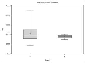
The second example (5_17 from your textbook) is new. It has to do with the life expectancy of light bulbs.  A person has to buy a large shipment of bulbs. She first buys 40 of each brand and subjects them to an accelerated life test to determine which last longer. This is a two-tailed test because before the test we have no particular expectation of which brand might be better.

The input is relatively simple and straight forward. However, remember, when inputting an external file with INFILE, a CSV file needs the options dlm=’,’ and dsd. A TXT file does not need either of these options and won’t work properly if they are present. Pay attention to which type of file you are inputting.

Class variables are sometimes called categorical, group or dummy variables. A variable that is going to represent classes can be either a numeric or a character variable. Either one will become a class variable when placed in a SAS class statement. When dealing with “class” variables, it is not unusual that they will be character variables and will need that “$” sign in input and length statements.

data bulbs;

   INFILE 'datatab_5_17.txt' missover firstobs=2;

   input brand $ life;

datalines; run;

;

run;

Once the data was input the two-tailed t-test is relatively straight forward.

PROC ttest data=bulbs;

   CLASS brand;

   VAR life;

   title2 "The two-sample t-test";

   TITLE3 'Two-tailed hypothesis';

RUN;

The results of the Folded F test indicated a highly significant difference in the variances (, P<0.0001). The variances were therefore not pooled. The resulting test of the means, using a Satterthwaite adjustment due to unequal variances, indicated a significant difference between the means (, P=0.0204). Note that when the Satterthwaite adjustment is used the degrees of freedom are not usually round integer values.

Method           Variances         DF    t Value    Pr > |t|

Pooled              Equal           78       2.41      0.0184

Satterthwaite    Unequal      42.882       2.41      0.0204

Equality of Variances

Method        Num DF     Den DF     F Value     Pr > F

Folded F          39          39        20.05     <.0001

Finally, I requested a univariate analysis of the sorted data. Here, my objectives were to obtain confidence intervals and tests of normality. Since there are two datasets, and the variances are not equal, we will need to examine each separately for normality, hence the “BY” statement. 

proc sort data=bulbs; by brand; run;

PROC UNIVARIATE data=bulbs normal plots CIBASIC; by brand;

VAR life;

ods exclude BasicMeasures ExtremeObs Quantiles Modes

 ExtremeValues MissingValues TestsForLocation;

RUN;

When the PROC UNIVARIATE is run with a BY statement, the procedure provides side-by-side box plots for comparison. It is clear that one of the two samples has what appears to have a larger variance and a possible outlier (i.e. an excessively large or small observation).

The results of the confidence interval request and test of normality for the first dataset are given below.

Basic Confidence Limits Assuming Normality

Parameter          Estimate     95% Confidence Limits

Mean                     1532           1416         1648

Std Deviation     362.78824     297.18198   465.83298

Variance              131615          88317       217000

Tests for Normality
Test                  --Statistic---    -----p Value------

Shapiro-Wilk           W     0.950104    Pr < W      0.0765

Kolmogorov-Smirnov    D     0.103259    Pr > D     >0.1500

Cramer-von Mises      W-Sq   0.06043    Pr > W-Sq  >0.2500

Anderson-Darling      A-Sq  0.419408    Pr > A-Sq  >0.2500

Both the first and second data set showed similar results for normality (not rejected) but an apparently smaller level of variability in the second data set. 

Basic Confidence Limits Assuming Normality

Parameter          Estimate     95% Confidence Limits

Mean                     1390           1365         1416

Std Deviation      81.03021      66.37679   104.04566

Variance                6566           4406        10826

Tests for Normality

Test                  --Statistic---    -----p Value------

Shapiro-Wilk           W     0.956297    Pr < W       0.1250

Kolmogorov-Smirnov    D     0.138372    Pr > D       0.0517

Cramer-von Mises      W-Sq  0.072289    Pr > W-Sq  >0.2500

Anderson-Darling      A-Sq  0.473393    Pr > A-Sq   0.2358

Based on the graphics, the observations range from about 1200 to 1500 in data set “b” and from about 900 to 2700 in data set “a”, but only one value in the second data set is much over 2000.  Recall that the t-test for these two data sets showed a significantly difference variance (P<0.0001) and a significant difference in the means (P=0.0204).  I was curious if the large variance and significant difference could be caused entirely by the single potential outlier.  I removed the outlier by including in the data step the statement.

if life gt 2500 then delete;

This will remove any observation with a value of life greater than 2500, but of course only one value that is that large; the suspected outlier. The conditional options that can be used in an if statement are the following (gt for greater than, lt for less than, ge for greater than or equal, le for less than or equal, eq or equal and ne or not equal). 

After removing the potential outlier the results were as follows: 

Method         Variances           DF    t Value    Pr > |t|

Pooled              Equal           77       2.18       0.0320

Satterthwaite    Unequal      43.056       2.16       0.0364

              Equality of Variances

Method      Num DF    Den DF    F Value    Pr > F

Folded F        38        39      14.60    <.0001

The overall results actually did not change. The hypotheses of equal variances and equal means are still rejected.  The variances are somewhat closer and the F test statistic has fallen from 20 to 14, but the resulting test indicates that the variances are still highly significantly different (, P<0.0001). 

Assignment 9

The first dataset for the assignment (Exercise 5.1, Table 5.12 from Freund, Rudolph J., William J. Wilson and Donna L. Mohr. 2010. Statistical Methods. Academic Press (ELSIVIER), N.Y.) is data for a statistics class with two sections that were each taught with different methods. We want to test the hypothesis that the test scores for the first method (a) are higher than the second (b).  You do not need to output two datasets or arrange a “univariate” type data set, the data already comes that way. 

Answer all questions about hypothesis tests by stating the outcome (REJECT the null hypothesis or FAIL to reject the null hypothesis) and Give a P-value where a relevant P-value is available. Turn in your log and the list output or results viewer output. You may write answers to questions on the log, or on a separate page. 

Task 1: Run a one-tailed two-sample t-test against the upper tail of stat teaching method “a” versus stat teaching method “b” (e.g. or ). Note that by default SAS will subtract the second name in alphabetical order from the first (e.g. meanA – meanB) ..................................................  (1 point)

Question 1: If there is not a statistically significant difference between the variances then they can be pooled. Should the variances be pooled for this analysis? .........................................................  (1 point)

Question 2: Is there a significant difference between the means? ...................................................  (1 point)

Task 2: Your second dataset (Exercise 5.13, Table 5.19) examines the half-life of a two drugs of the class Aminoglycosides, Amikacin and Gentamicin, coded as A and G respectively. This will be a two-tailed t-test. In addition to testing the means for equality we will check the assumption of normality. 

Task 2: Do a two sample t-test of the differences between the drugs. ............................................  (1 point)

Question 1: If there is not a statistically significant difference between the variances then they can be pooled. Should the variances be pooled for this analysis? .........................................................  (1 point)

Question 2: Is there a significant difference between the means? ...................................................  (1 point)

Task 3: Finally, using the dataset from Exercise 5.13, Table 5.19, sort by the two drugs and run a PROC UNIVARIATE analysis BY the drug variable producing two outputs, one for each drug.  Include in the univariate analysis the confidence intervals, plots and test of normality. ............................  (1 point)

Question 5: Is the hypothesis of “normality” rejected for either of the two samples? .....................  (1 point)

Question 6: Do the bounds on the confidence interval for the standard deviation appear to be just the square root of the bounds on the confidence interval limits of the variance or is some other calculation involved?      (1 point)

Task 4: Prepare a PROC BOXPLOT for the two classes of the second data set. ...........................  (1 point)