EXST SAS Lab

Lab #7: Hypothesis testing with
Paired t-tests and One-tailed t-tests

Objectives

1. Infile two external data sets (TXT files)

2. Calculate a difference between two variables in the data step (Dataset 1)

3. Use PROC UNIVARIATE to do a paired t-test (Dataset 1)

4. Use PROC TTEST to do a paired t-test (Dataset 1)

5. Test the assumption of normality with PROC UNIVARIATE (Dataset 1)

6. Use PROC TTEST to do a one-sample t-test (Dataset 2)

7. Test the assumption of normality with PROC UNIVARIATE (Dataset 2)

The datasets

The datasets are from the textbook (Freund, Rudolph J., William J. Wilson and Donna L. Mohr. 2010. Statistical Methods, Academic Press (ELSIVIER), N.Y.). The text book offers datasets as EXCEL and TXT, but not as CSV. A text data set (TXT) has values that are separated by blank spaces (one or more, it makes no difference). Inputting an external text file is exactly the same as the previously discussed CSV files except you do not need to specify a separator because blank spaces are the SAS default. The infile statement needs only the file name and firstobs=2 if the first line has the variable names.

I would usually include MISSOVER, but it won’t be necessary in this case. The missover option prevents SAS from going to the next line if it does not find a value for every variable on the current line. For example, the first data set discussed below has two variables on each line of data (AreaA and AreaB). If SAS only found one value on some line, what should it do; either (a) call the second value missing (represented in SAS by a dot, “.”) or (b) go to the next line and take the first value it finds and use that as the value of the second variable. The default is (b), to go to the next line. That is something I almost never want it to do. Missover prevents that behavior and goes with option (a).

PROC UNIVARIATE

As we have already seen, PROC UNIVARIATE is an important procedure that provides a great deal of information, sometimes more than we want or need. Below are some important additional things to know about this procedure.

• Multiple occurrences of observations are indicated to PROC UNIVARIATE with a FREQ statement instead of a WEIGHT statement. When available to a procedure, the FREQ statement always represents multiple numbers of observations per record (i.e. n_i). The total number of observations would be the sum of all n_i. The WEIGHT statement sometimes (e.g. PROC REG) gives more or less emphasis to some records while still representing only a single observation.
• It is possible to test a distribution for normality with PROC UNIVARIATE. These tests are requested with a NORMAL option in the PROC statement. There are usually 4 tests given, sorted from best (on top) to worst. The Shapiro-Wilks’ test is by far the best, but is only available for sample sizes less than 2000. When unavailable, the Kolmogorov-Smirnov is the second best choice; a distant second best IMHO. The null hypothesis for these tests is that the observed data is consistent with a normal distribution. The alternative is that the observed data does not conform well to a normal distribution.
• Useful graphics (stem & leaf and box plots) can be requested with the PLOT option in the PROC statement. If the hypothesis of a normal distribution is rejected, these plots can help understand why the data is not well fitted by a normal distribution. (e.g. outliers, skewed, polymodal, etc).
• Other statistics that can be requested on the PROC statement include CIBasic to estimate confidence intervals on the mean and variance, and modes which will provide a list of modes when more than one mode exists.
• Sometimes PROC UNIVARIATE gives more information than is needed. There are ODS options available to suppress default sections of the output. The following statement would suppress all default output, giving nothing unless something like normal, plot or CIBasic was requested.

ods exclude BasicMeasures ExtremeObs ExtremeValues Modes
     Moments MissingValues Quantiles TestsForLocation;

In this exercise we will use PROC UNIVARIATE to do a paired t-test. By default, the univariate procedure automatically tests the mean against zero (unless suppressed by “ODS exclude TestsForLocation”). All that is needed to do a paired test is to take the paired values and calculate a difference (d_i) between the members of each pair in the data step (). The procedure will then test the mean difference against zero. The null hypothesis is, where,, is the population mean difference. The alternative hypothesis is the non-directional, two-tailed alternative, . There is no directional alternative (e.g.  or ) with PROC UNIVARIATE.

P-values: Both the t-test of the mean and the test for normality in PROC UNIVARIATE yield P-values. All P-values work pretty much the same way; we are going to reject the null hypothesis when we observe an unusual event (i.e. a low probability of occurrence if the null hypothesis is true). In testing normality the hypothesis is that the observed data is consistent with, or representative of, a normal distribution. As usual, rejection occurs when the P-values is less than (or equal to?) your chosen value of a, usually 0.05. The alternative hypothesis is that the observed distribution is not consistent with what would be expected for a normal distribution. For the t-test, a value of greater than your chosen value of a would indicate a result consistent with the null hypothesis, while a P-value smaller than a would indicate an unusual event and suggest the alternative hypothesis is the more likely case. 

Examples

The first example dataset from your textbook is Table5.13 (see Freund, Wilson and Mohr datasets, datatab_5_13.txt). The data consists of air pollution index measurements for two areas of the city on eight randomly selected dates. The areas are tested on the same date, so the data is considered to be paired by date. Although this example is not intended to be a one-tailed example, we will use it to test both one and two-tailed alternatives for comparison.

We will test the two-tailed alternative first using PROC UNIVARIATE , and simultaneously test for normality. The variables in this dataset are AreaA and AreaB. The difference to be tested as a paired t-test should be calculated in the data step as DIFF = AreaA – AreaB. Then the differences it tested in as follows:

proc univariate data=Pollution plot normal CIBasic;

   var diff;

   ods exclude extremeobs quantiles;

run;

This procedure will automatically test the “Location” of the variable DIFF against zero. Additionally, since we requested the options plot and normal on the PROC statement, the procedure will test for normality and produce a normal probability plot. Interpretation of the test of normality is discussed above. Confidence intervals were also requested. These will be discussed in class. Titles have been removed from the SAS code here, but are available in the posted example program.

The test for location is the first t-test to examine. The student’s t-value is given as 14.49. The analysis indicates that, if the null hypothesis is true, a value of 14.49 with n – 1 = 7 degrees of freedom would occur with a probability of <0.0001, or less that once in 10,000 attempts. This is pretty solid evidence that the null hypothesis,, is not true and can be rejected in favor of the alternative, .

Tests for Location: Mu0=0
Test	Statistic		p Value
Student's t	t	14.49172	Pr > |t|	<.0001
Sign	M	4	Pr >= |M|	0.0078
Signed Rank	S	18	Pr >= |S|	0.0078

The best test of normality is given by the Shapiro-Wilk statistic. In this case the results indicate that a statistic value of 0.921 would occur about 44% of the time in the null hypothesis is true. A value that occurs nearly half the time by random chance is not one that gives evidence that the distribution is not consistent with the null hypothesis of normality. We would conclude that the observed distribution of values may indeed come from a normal distribution. Of course, this is just the best evidence we have; we can never be 100% sure.

Tests for Normality
Test	Statistic		p Value
Shapiro-Wilk	W	0.92124	Pr < W	0.4400
Kolmogorov-Smirnov	D	0.261203	Pr > D	0.1049
Cramer-von Mises	W-Sq	0.062716	Pr > W-Sq	>0.2500
Anderson-Darling	A-Sq	0.361255	Pr > A-Sq	>0.2500

PROC TTEST

This procedure has a number of options and statements to facilitate both one sample and two sample t-tests. Some of the available statements and options are:

• A CLASS statement specifies the qualitative or categorical or group variable that distinguishes between the two samples to be tested in a two-sample t-test.
• The VAR statement names the quantitative variable to be tested in the t-test.
• The PAIRED statement specifies the name of two different variables that are entered on the same record and are members of a pair for the paired t-test. When a PAIRED statement is used the PROC TTEST cannot also have a CLASS or VAR statement.
• The option ALPHA= is used to specify an alpha value to determine level of confidence for confidence intervals. When not specified, a default value of a = 0.05 is assumed.
• The H0= option can be used to specify a hypothesized value. If not specified, a default value of zero is assumed.
• The SIDES= option specifies the number and direction of sides. A two-tailed test is assumed when this option is not included.

The second part of the first example is to do a one-tailed test with PROC TTEST. Here again the null hypothesis is a test against zero. PROC TTEST can either test DIFF against zero or can take the paired values and test for a difference without calculating a difference in the DATA step. We will also pretend that we are testing a one tailed alternative where we suspect that values of pollution in AreaA are higher than in AreaB. If we subtract AreaB from AreaA then we will hypothesize that the result will be greater than zero (the upper tail) and tests accordingly. PROC TTEST also has a “PAIRED” statement that allows for directly testing a paired difference without calculating that difference previously in the data step. The PROC TTEST statements for the two approaches are:

PROC ttest data=Pollution sides=u;

VAR diff;

run;

PROC ttest data=Pollution sides=u;

PAIRED AreaA * AreaB;

run;

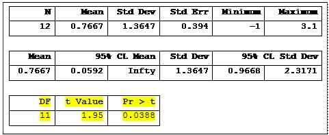
A comparison the output from the two approaches shows identical results. The t-value of 1.95 with 11 d.f. would be expected to occur only 3.88% of the time if the null hypothesis is true. As a result, if our rejection level was set at the usual convention, a = 0.05 or 5%, we would reject the null hypothesis and conclude that there was a significant difference between the two areas.

Testing against an hypothesized value other than zero

In a second example we will test 12 values of systolic blood pressure against a hypothesized value of 129 ( where m_o = 129 mm). This test is also a one-tailed test () since the values are drawn from a population of males whose dietary habits are suspected of causing high blood pressure (textbook exercise 4.6).

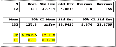
PROC ttest data=SystolicBP sides=u ho=129;

VAR BP;

run;

The HO= option is SAS allows the direct testing of data against a value other than zero. I would also be valid to subtract the hypothesized value of 129 from every value and then test against zero.

Finally we want to examine the assumption of normality for the second data set. This test can be done in PROC UNIVARIATE with the following statements. Note that the statements below produce output for the tests of normality and the plots with all other output suppressed.

proc univariate data=SystolicBP plot normal;

var BP;

ods exclude BasicMeasures ExtremeObs ExtremeValues Modes

       Moments MissingValues Quantiles TestsForLocation;

run;

Interpretation of the test of normality is discussed in detail in the previous exercise. The assumption of normality would not be rejected

Assignment 7

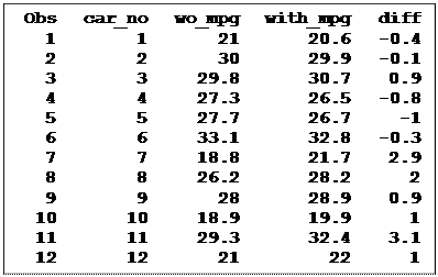
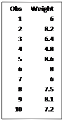
This assignment uses two data sets. The first is paired data resulting from testing a dozen cars, each with and without a device intended to improve mileage (textbook table 5.15). The second is a set of 10 values of weights of infants 12 hours after birth, healthy – but from low income neighborhoods (textbook exercise 4.9). The objective in both cases it to conduct a t-test of the variable of interest and to also test the assumption of normality. Complete the following assignment and turn in a print of your LOG and your results from either the OUTPUT or RESULTS viewer window.

The objective of the first exercise is to test the effectiveness of a device that may increase a car’s mileage. Twelve cars were used in the study in random order and each was run on a standard course with and without the device, also in random order. The data is from table Table 5.15. The variables are CarNumber, MileageWith and MileageWithout.

1) You will want to include in your program the “usual statements” with option, comments and titles similar to those in previous assignments as well as appropriate title statements.

2) The datasets is stored as a TXT files dataset. Input the dataset as an external dataset using code similar to the infile statement of a CSV file with the modifications discussed above.

3) The test to see if the new device affects mileage could be done as a one-tailed test or as a two-tailed test. Since we cannot do one-tailed tests of means with proc univariate, we will do a two-tailed test first. To do this you will need to calculate a difference between the two variables in the data step. Conveniently, they are on the same record, so you need only calculate a difference in the data step. Assuming it would be convenient for a positive difference to indicate a positive effect (i.e. the device improves mileage) we would subtract the mileage “without” the device from the mileage “with” the device. Do it!  (1 point)

4) Use proc univariate to do a two-tailed paired t-test of  versus
Include the options plot, normal and CIBasic on the plot statement and use an ods statement to exclude extremeobs and quantiles. (1 point)

Question 1: Using PROC UNIVARIATE would you reject?  (1 point)

Question 2:  Using PROC UNIVARIATE would you reject the null hypothesis that the distribution of the observed data is consistent with a normal distribution?  (1 point)

Now we want to test to see if the new device improves mileage using PROC TTEST. This procedure can do one-tailed tests, and this is probably closer to the original intent of the problem; testing to see if the new device improves mileage. PROC TTEST has mechanisms for handling data on the same record or different records, so we can either test the difference we calculated in the data step, or test the original paired variables directly. We will do both.

5) Use proc TTEST to do a one-tailed paired t-test of  where, versus, so the alternate hypothesis indicates that the device improved mileage. Use the difference calculated previously to test the hypothesis.

Question 3: Using PROC TTEST and a one-tailed test, would you reject the null hypothesis?  (1 point)

Question 4: Are the results for question 1 and question 3 the same? If not, why not. (1 point)

6) proc TTEST has a paired statement and can do a one-tailed paired t-test like the above directly on the two variables without calculating a difference in the data step. Repeat the one-tailed test of paired data using the paired statement instead of the calculated difference.

Question 5: Are the results of the two one-tailed paired t-test in tasks 5 and 6 the same? If not, why not. (1 point)

The second dataset is a small set of 10 observations of infant weights at 12 hours after birth. We want to conduct a one tailed test of these values against a hypothesized value of 7.5 lbs. This will be a one tailed hypothesis because we believe the infants may weigh less that the norm since they are from a low income neighborhood.

7) Do a one-tailed one-sample t-test of  versus  where m_o = 7.5 lbs. Notice that you are testing against the lower tail in this task. “L” is for lower.

Question 6: Using PROC TTEST and a one-tailed test, would you reject the null hypothesis?  (1 point)

8) Finally, test the assumption of normality with PROC UNIVARIATE. Produce output only for the tests of normality and the plots with all other output is suppressed.  (1 point)

Question 7: Would you reject the null hypothesis that the distribution of the observed data is consistent with a normal distribution?  (1 point)