EXST SAS Lab

Lab #6: More data step tasks

---

Objectives

1. Working from an current folder

2. Naming the HTML output data file

3. Dealing with multiple observations on an input line

4. Creating two SAS work files from one input file

5. Outputting a data set from a procedure

6. Plotting means from an output dataset

7. Confidence intervals (μ, σ. and σ²)

The current folder

As we saw in assignment 4, it is often advantageous to work from within a new directory created specifically for that programming task. This assignment will deal with several data sets and it will be advantageous to use a separate folder as the “current folder” to manage the files.

As you may recall, SAS keeps track of the last folder when a SAS editor is run by double-clicking on a file name. The directory from which the program was launched from is called the “current folder” and is listed in the lower, right margin of the SAS window. If you wish to change the current folder you can double-click on the folder name and change the folder. If the data for a program is stored in the current folder, then it is not necessary to list all the subdirectory information to access the file, it is only necessary to call up the file by giving just the file name. Also, any ODS output from the program will be automatically stored in the current folder without specifying the complete subdirectory information.

Set up a new subdirectory on your flash drive or in “My Documents”. The full path for me would be “C:\Users\Lecture\Documents\My SAS Files\EXST 700X Assignment 06”. Then, copy the materials for today’s program into that directory including the data files and a program file you create called ASSIGNMENT06.SAS, or some name of your choice. As long as you launch this SAS program from the new directory, and as long as that directory remains the current folder, you may call up data by specifying only the filename – you do not need the whole path. Also, if you write HTML or RTF files with the ODS statement, you only need to specify the filename, not the full path, and it will be placed in this directly. It is therefore easy to keep all files associated with the programming task in a single directory.

If you set up an current folder as described above, you will find that the code we have been using to clear the Results Viewer “ods html close; ods html;” writes a file called “sashtml.htm” to the directory. With each additional run, SAS adds another file (sashtml2.htm, sashtml3.htm, sashtml4.htm, …). The following code can be used to have SAS write only one file, and to replace that file each time the program is run with the newest version of the output.

ods html close; ods html style=minimal body='EXST700X Assign06.html';

Note the minimal style request (a personal preference). It prevents SAS from adding various fonts and shading to the HTML document. The “BODY =” option causes SAS to write the Results Viewer file to a file named Assign06.html. After each run this file will contain the newest results of the SAS program output.

The datasets for today’s exercise is from the textbook (Freund, Rudolph J., William J. Wilson and Donna L. Mohr. 2010. Statistical Methods. Academic Press (ELSIVIER), N.Y.). The example dataset is from an experiment on the quality of steel. There are two categorical variables, CLEAN (concentration of cleaning agent) and TEMPR (an index of temperature and pressure). The variable to be analyzed is the ELAST, an index of steel quality. The dataset is available as either a TXT dataset (STEEL.TXT = space separated) or as a CSV file (STEEL.CSV = comma separated). You can use either one.

There are two common ways to set up data when there are multiple variables involved. One is to put each variable in its own column. This is sometimes called a “multivariate” arrangement since many multivariate analyses used data entered in this fashion. An alternative is to have all the values of particular variable in a single column with additional column to specify which category corresponds to that line.

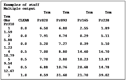
We do not have multivariate data. The table actually shows aspects of both a multivariate type of data table, where the TEMPR variable is arranged in columns, and a univariate type of data set with the levels of the CLEAN variable listed in a column. However, the two-way table above illustrates one problem faced in univariate analyses. We want to analyze and compare the steel quality variable (ELAST) in a univariate analysis. To do that we need a single variable column for the values of ELAST matched in a two other columns with the corresponding values of the variables CLEAN and TEMPR.

The task, then, is to get all those values of steel quality (ELAST) in a single column. We also need for the two categorical variables, CLEAN and TEMPR to each be in its own column. The resulting dataset has only those three variables and this would allow us to use our univariate analyses with sorts and BY statements, or to prepare graphics, or to analyze the data with procedures that have class statements, such as MEANS.

In this exercise we will read one data set that is a two-way table, and output two data sets, one a two-way table like the original and a second data set appropriate for univariate analysis. This can be done in a DATA step with two SAS output data sets from a single input. Notice the two data set names (STEEL and UNI) in the single DATA statement in the example below.

data STEEL uni; INFILE 'steel.csv' dlm=',' dsd missover firstobs=2;

   input CLEAN TemPr020 TemPr093 TemPr165 TemPr238 TemPr310;

These statements will read a CSV dataset called “steel.csv” from the current folder and create two SAS work files called STEEL and UNI. To output the proper datasets we will need to use an OUTPUT statement. Since the input data file in is already in the two-way table form, we can output each line directly to the two-way style dataset (STEEL) as it is read. The statement is simply “output steel;” following the input statement.

The output for the univariate dataset is a bit more complicated. Having read the first line from the external dataset we have the following line of data below (with headers added).

clean	tempr020	tempr093	tempr165	tempr238	tempr310
0	6.5	6.8	2.55	1.89	1.59

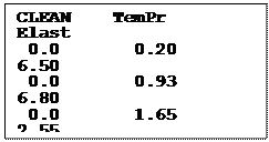
All of the numbers are values of ELAST except the value of CLEAN. We want to leave the value of CLEAN at “0” and output the 5 values of ELAST to 5 separate lines of data, each with the corresponding value of TEMPR (0.20, 0.93, 1.65, 2.38 and 3.10). We can output the 5 values with the 5 following lines of SAS code. Read one line of data, output five lines of data, one for each level of TEMPR.

      TemPrID = 'A'; TemPr = 0.20; Elast = TemPr020; output uni;

      TemPrID = 'B'; TemPr = 0.93; Elast = TemPr093; output uni;

      TemPrID = 'C'; TemPr = 1.65; Elast = TemPr165; output uni;

      TemPrID = 'D'; TemPr = 2.38; Elast = TemPr238; output uni;

      TemPrID = 'E'; TemPr = 3.10; Elast = TemPr310; output uni;

On the first line of code we set the value of TEMPR to the value 0.20 (the first TEMPR value in the table) and we set ELAST equal to the corresponding value of tempr, which is TEMPR020. Then, output this observation to dataset UNI creating the first line of the univariate dataset is as “0    0.20    6.50” for CLEAN, TEMPR and ELAST respectively.

On line 2 we set the value of TEMPR equal to the value 0.93, the second TEMPR value, and we set ELAST equal to the value read as TEMPR093. We then output this observation to dataset UNI. Note that CLEAN is still equal to 0, so the second line of the dataset is as “0    0.93    6.80”.

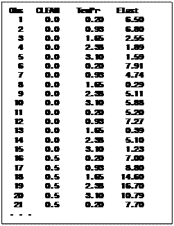
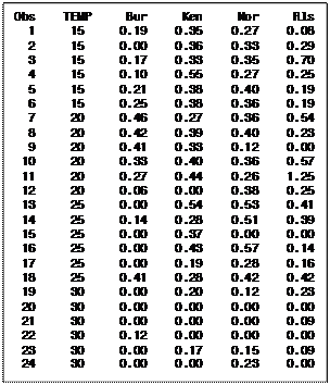
On line 3, we set the value of TEMPR equal to the value 1.65, ELAST equal to the value stored in the variable TEMPR165 and then output to dataset UNI. The third line of the dataset is UNI as “0    1.65    2.55”. Doing the same for the next two lines results in the first 5 lines of the dataset UNI shown to the right.

SAS then reads the second line of data from the source dataset and obtains the following values.

clean	tempr020	tempr093	tempr165	tempr238	tempr310
0	7.91	4.74	0.29	5.11	5.88

Again, this line is output directly into the STEEL SAS work file and the process is repeated, outputting 5 additional lines to the dataset UNI. The cycle is repeated until SAS has processed all the line of data in the original data set. The first 25 lines of the final UNI dataset is on the given below. This type modification of data sets is a frequent necessity that we will see later in the semester on some data sets used in Analysis of Variance.

An additional variable (TemPrID) was added to the dataset because the steel data (example data set) set did not have a categorical variable suitable for use as an identifier in graphics. The Potato data set (assignment data set) has character variables for the potato varieties so you will not need to create an identifier variable.

One more comment on the creation of these data sets. When the data set STEEL was output the only variables that were on the data set were the ones that were to be part of STEEL; CLEAN, TemPr020, TemPr093, TemPr165, TemPr238 and TemPr310. These were output. Then for the data set UNI we used the variable CLEAN and created the variables TemPrID, TemPr and Elast. However, at the point that we output UNI the variables for STEEL were still on the data set and would also be included in the output. There are two options for removing the extra variables. One is a DROP statement where the variables to be excluded are listed after the word DROP. The other is a KEEP statement that specifies the variables to keep in the data set. The DROP and KEEP statements can be separate statements. However, since two data sets being produced in this case, the best placement of the KEEP statement is as part of the data step.

data STEEL (keep = CLEAN TemPr020 TemPr093 TemPr165 TemPr238 TemPr310)

      uni    (keep = CLEAN TemPrID TemPr Elast);

SAS supports “do loops: and there are more “elegant” ways of outputting multiple lines from a single line of input. However, the approach given above is the simplest and most straight forward.

Two additional procedures, a proc print and a proc means with a class statement, are included in the program and requested in the assignment. These are not new and are not discussed here.

Outputting a data set from a procedure

For the next task the data set must be sorted by the category variables (CLEAN and TEMPR). Proc MEANS is then run on the variable ELAST with a BY statement. This creates a mean for every combination of the category variables. A NOPRINT option is also included. Obviously, with the noprint option, no printed or listed output is produced. So a Proc MEANS with a NOPRINT option is a waste of time unless some other mechanism is used to get output, like the output statement.

Most SAS procedures have an OUTPUT statement option. In PROC MEANS the output statement produces a new SAS dataset with selected statistics. The output statement used in the example created a new SAS work data set and caused requested statistics to be output (n, mean, var, std and stderr).

proc sort data=uni; by clean TemPr TemPrID; run;

proc means data=uni noprint; by clean TemPr TemPrID;

var Elast;

output out = next1 n=n mean=mean var=var std=std stderr=stderror;

run;

The value to the left of the equal sign is the SAS key name of the statistic and the name on the right can be any name you wish to specify. I often use the same name.

This output dataset can now be used in various ways. A print of the means for each combination of CLEAN and TEMPR is an efficient way of expressing this information where a table of means, standard errors and other statistic are needed.    

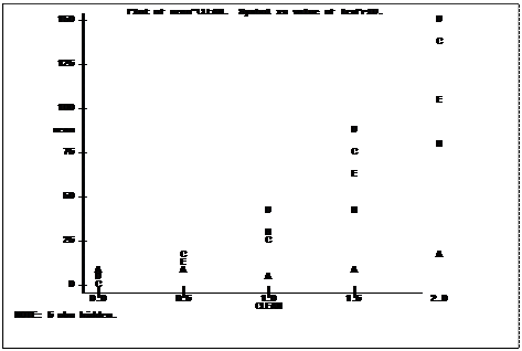The means can also be used in other SAS procedures. For example, PROC PLOT is used to produce a scatter plot of the means. In this plot the MEAN of each combination of CLEAN and TEMPR data is plotted on the Y axis and the quantitative variable CLEAN is used as the X axis. Setting the plot statement equal to a variable means that the characters used to represent the observations on the plot will be equal to the first letter of the variable. The ID variable TEMPRID, with values A through E for the values of TEMPR (0.20, 0.93, 1.65, 2.38 and 3.10), can be used to identify the points in the scatter plot. If I had used the variable TEMPR instead of creating an ID variable the characters would have been (0, 0, 1, 2 and 3) and we would not be able to distinguish between level 0.20 and 0.93 since both would be represented by a “0”..

proc plot data=next1;

plot mean*clean=TemPrID; run;

One last procedure was run to obtain confidence intervals for the mean, variance and standard deviation of the variable ELAST. This can be done in PROC UNIVARIATE if the CIBASIC option is put on the PROC statement.

PROC UNIVARIATE data=uni CIBASIC;

VAR elast;

ods exclude BasicMeasures ExtremeObs ExtremeValues Modes

                 MissingValues Quantiles TestsForLocation;

RUN;

The proc univariate statement produces a lot of output. If some of this output is not wanted, it can be suppressed with an ODS exclude statement listing those sections that are not desired. The selection in the statement above suppresses all output except the moments section. There are also some sections that are not included by default. The cibasic option, requested above to get confidence intervals, is one of these. Other frequently used options are plot and normal.

Note that the mean and confidence intervals calculated here are for all values of ELAST, averaged across all levels of CLEAN and TEMPR. Eventually, we will use Analysis of Variance to determine if there are statistically significant differences in the various levels of these variables. Based on that information we may combine the estimates and confidence intervals, or we may prefer to keep them separate.

SAS Help

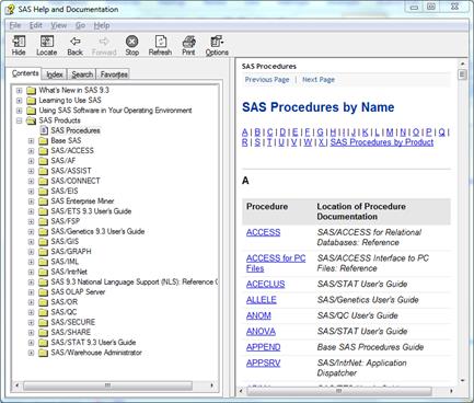
There are several procedures and SAS statements used in the program above that potentially involve long lists of options. Rather than try to remember options like the statistics that can be requested in PROC MEANS, I would encourage you to explore the SAS help procedure.

Rather than employ the SAS search option, find the “SAS Procedures” list in the help window. Then choose the procedure of interest.

Under the PROC MEANS link, for example, in the section for “statistic-keyword(s)” are the following keyword options: “CLM, NMISS, CSS, RANGE, CV, SKEWNESS|SKEW, KURTOSIS|KURT, STDDEV|STD, LCLM, STDERR, MAX, SUM, MEAN, SUMWGT, MIN, UCLM, MODE, USS, N, VAR, P1, P5, P10, P20, Q1|P25, P30, P40, MEDIAN|P50, P60, P70, Q3|P75, P80, P90, P95, P99, QRANGE, PROBT|PRT, T.” In this section SAS also lists the default statistics as “N, MEAN, STD, MIN, and MAX”.

It is much easier to learn to use SS help rather than try to remember lists like this.

Citation for SAS online documentation:

SAS Institute Inc. 2011. SAS OnlineDoc® 9.3. Cary, NC: SAS Institute Inc.

Assignment 6

I recommend you explore the benefits of using the “current folder” for data input and output; eliminating the need to specify the full directory. However, this is optional.

Task 1: Create an HTML output file using the ODS HTML statement (minimal or not, your choice, current folder of full path, also your choice). (1 point)

Task 2: Input the data from either POTATO.csv or POTATO.txt and output two data sets, one like the original dataset (table to the right) and a second dataset with one variable for TEMP, one for VARIETY and one for POUNDS. (2 points)

If you find this task to be too arcane and not worth the two points, you may use the dataset Table 9_29.csv or Table 9_29.txt which is already set up as a “univariate” file. This will allow you to finish the assignment.

Task 3: Print the multivariate type dataset. Do not print the univariate data as it takes too many pages. (1 point)

Task 4: Run PROC MEANS with a class statement, obtaining a value of “n” an estimates of the mean and standard error for each combination of TEMP and VARIETY. (1 point)

Task 5: Sort the data by TEMP and VARIETY and run PROC MEANS by TEMP and VARIETY. Make sure to include a NOPRINT statement and to OUTPUT the statistics n, mean, var, std and stderr. (2 points)

Task 6: Print the output dataset from the PROC MEANS. (1 point)

Task 7: Plot the means from the PROC MEANS OUTPUT, plotting the mean on the quantitative variable TEMP and using VARIETY as a category indicator for each mean. (1 point)

Task 8: Run PROC UNIVARIATE to get the confidence interval for the mean, variance and standard deviation for the potato weights. Suppress all other output except the MOMENTS section. You will only need one confidence interval for all observations; you do not need separate estimates and intervals for each combination of TEMP and VARIETY. (1 point)