Lab #1: Introduction to Basic SAS Operations
Getting Started: OVERVIEW OF SAS (access lab pages at http://www.stat.lsu.edu/exstlab/)
 There are several ways to open the SAS program. You
may have a SAS icon on your desktop that will open SAS, or you can open SAS
from the start menu. If you use windows file explorer, double clicking on a SAS
file will open the file in SAS. However, depending on the way your computer is set
up, it may open in SAS Enterprise instead of SAS 9.3 or 9.4. Please make sure
that when you open SAS you are using SAS 9.3 or 9.4 and not SAS Enterprise.
There are several ways to open the SAS program. You
may have a SAS icon on your desktop that will open SAS, or you can open SAS
from the start menu. If you use windows file explorer, double clicking on a SAS
file will open the file in SAS. However, depending on the way your computer is set
up, it may open in SAS Enterprise instead of SAS 9.3 or 9.4. Please make sure
that when you open SAS you are using SAS 9.3 or 9.4 and not SAS Enterprise.
Recommendation 1: Most future labs will be introduced with a video. You should view the video before class or bring earphones to lab in order to follow the video during the lab session.
Recommendation 2: You should establish a subfolder in your “documents” or “desktop” folder for each lab assignment. You should then frequently save your program to that subfolder. As old programs may be used as the basis of future programs, it is also recommended that you save your SAS assignment files from week to week. Finally, since you may not be using the same machine every week, you should save your file to a flash drive, tigerbytes or email a copy to yourself.
SAS PROGRAMMING
There are three main windows in SAS: Program Editor, Log, and Output.
· Program Editor: where you create your SAS program.
· Log: gives you information about possible errors after you have run your SAS program.
· Output: gives you a listing of the results of successful SAS program.
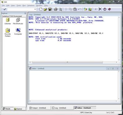
The graphic to the right shows the PROGRAM window in the lower right and the LOG window in the upper right. The output window is hidden behind these and can be viewed by clicking on the “Output” tab at the bottom. The tall window to the left can access either the SAS explorer or the Results listing by using the two tabs at the bottom of that window.
A SAS program usually consists of the following parts:
- optional statements to control output, “housekeeping” statements
- a data statement
- one or more PROC steps (procedures)
More detail is given in the demonstration below.
SAS Demonstration
Our first task will be to create a small dataset and “print” that dataset to the output window. SAS programs usually start with a DATA step where the dataset is created. Once the dataset is available, various procedures can be run on the dataset.
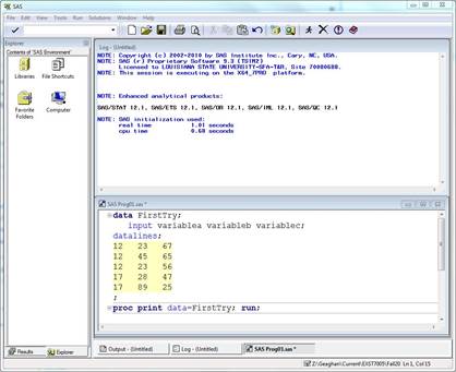
The demonstration program below is written in the SAS Program window. The program creates a dataset called “FirstTry” with 3 variables (columns) and 5 observations (rows). Note that the values of the variables on each line are separated by one or more blanks. A few other things that you should note:
- All SAS statements end with a semicolon
- More than one SAS statement can be put on a line, or a SAS statement can continue across several lines, as long as every statement ends with a semicolon.
- Data listed as part of the program is also terminated with a semicolon. Data does not have to be entered in the program; it can also be read from files that are external to the SAS program.
 Once the dataset is
created, various SAS procedures (called PROCs) can be used to analyze the
data and present results. We will start with a listing of the data created
with a procedure called PROC PRINT.
Once the dataset is
created, various SAS procedures (called PROCs) can be used to analyze the
data and present results. We will start with a listing of the data created
with a procedure called PROC PRINT.
This program is called “SAS PROG01.sas”. The asterisk beside name in the upper left corner of the window and in the tab indicates that the program has been modified since it was last saved. When you create a SAS program you should save it often. During the class we recommend that you make a subdirectory in your “documents” directory for you lab program and output. However, since you may not have the same lab computer next week we also recommend that you save you program to a flash drive, Tigerbytes or email yourself a copy. Once the program is created you can run the program, or “Submit” the program, for execution. This can be done from the menus or from the icons in the top rows.
SAS Icons: SAS instructions can be given by either menu commands or from a series of icons at the top of the SAS window. The icon graphic below shows icons that complete the following commands in the order of the icons:
New; Open; Save; Print; Print preview; Cut; Copy; Paste; Undo; New Library; SAS Explorer; Submit; Clear all; Break; Help

The LOG window gives information on the execution of the program. If your program did not execute properly you should examine the log for error messages that may explain the failure. The program would then be modified if necessary, and rerun.
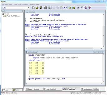
SAS creates a new window called the “Results Viewer” when the program is executed and produces output. This window is in HTML format and a new tab for the window is created below the left hand windows.
The program to this point consists of the following lines. These lines will read the data and print a listing of the data. You can copy the lines below, paste them in your SAS program window and submit the program.
data FirstTry;
input variablea variableb variablec;
datalines;
12 45 65
17 28 47
12 23 67
12 23 56
17 89 25
;
proc print data=FirstTry; run;
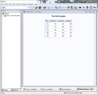
Note the output from the program.
|
The SAS System |
|||
|
Obs |
variablea |
variableb |
variablec |
|
1 |
12 |
45 |
65 |
|
2 |
17 |
28 |
47 |
|
3 |
12 |
23 |
67 |
|
4 |
12 |
23 |
56 |
|
5 |
17 |
89 |
25 |
The data can be sorted by adding the following lines to the program.
proc sort data=FirstTry;
by variablea variableb variablec;
run;
proc print data=FirstTry; run;
 The resulting output is sorted in order. The first
sort level is VARIABLEA where the three values of 12 are together followed by
the two values of 17. There were two values of 23 in VARIABLEB within the first level of VARIABLEA. When the VARIABLEB
is sorted the order of VARIABLEA is unchanged but when several observations of VARIABLEA are the same value the VARIABLEB is sorted within these values. Likewise, sorting by VARIABLEC after sorting by VARIABLEA
and VARIABLEB only sorts VARIABLEC
when there are several observations with the same values of VARIABLEA and VARIABLEB. Make
sure you understand how this hierarchy of sorts works. It will be relevant to
future work.
The resulting output is sorted in order. The first
sort level is VARIABLEA where the three values of 12 are together followed by
the two values of 17. There were two values of 23 in VARIABLEB within the first level of VARIABLEA. When the VARIABLEB
is sorted the order of VARIABLEA is unchanged but when several observations of VARIABLEA are the same value the VARIABLEB is sorted within these values. Likewise, sorting by VARIABLEC after sorting by VARIABLEA
and VARIABLEB only sorts VARIABLEC
when there are several observations with the same values of VARIABLEA and VARIABLEB. Make
sure you understand how this hierarchy of sorts works. It will be relevant to
future work.
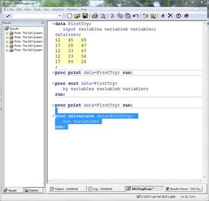 The last procedure to be executed in this exercise is
PROC UNIVARIATE. The code below applies the procedure only to the variable VARIABLEB. It can be run on any quantitative variable and it
could be run on several variables at the same time by listing several variables
in the VAR statement, which would provide a separate analysis for each
variable.
The last procedure to be executed in this exercise is
PROC UNIVARIATE. The code below applies the procedure only to the variable VARIABLEB. It can be run on any quantitative variable and it
could be run on several variables at the same time by listing several variables
in the VAR statement, which would provide a separate analysis for each
variable.
proc univariate data=FirstTry;
var variableb;
 run;
run;
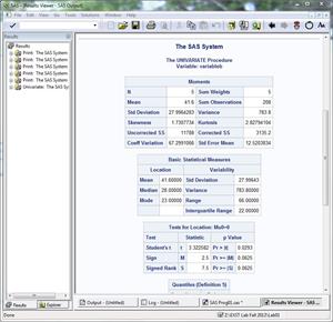
The results for PROC UNIVARIATE will be listed in the results viewer. The output from PROC UNIVARIATE will be important to the early part of this statistical methods class. It will provide measures of central tendency (mean, median, mode) and measures of dispersion (variance, standard deviation, range) as well as other basic statistics.
OPTIONAL STATEMENTS
There are a number of statements that can be included in the program that will simplify or modify the output. These are “housekeeping” statement that you may wish to include at the beginning of all your SAS programs.
dm 'log;clear;output;clear';
options nodate nocenter pageno=1 ls=78 ps=55;
OPTIONS FORMCHAR="|----|+|---+=|-/\<>*";
ODS listing; ods graphics off;
title1 "EXST 7005 Assignment 1";
1) The first statement above tells SAS to clear the log and output windows each time the SAS program is submitted. If not cleared successive “runs” of the SAS program accumulate in the output and log window with the newer output at the bottom.
2) The second statement allows you to specify some output options:
a) The ls= option changes the number of characters printed across the page, and can take on values between 64 and 256.
b) the ps= option changes the number of lines printed down the length of the page. The values shown above are typically good for 8.5 X 11" paper.
c) pageno=1 resets the starting page number at 1 each time the program is run.
d) The nodate and nocenter options suppress the listing of the date in the header line and the centering of output.
e) The “FORMCHAR” option specifies characters to be used for the line printer graphics from some procedures. The default characters are from SAS proprietary font, not available on all machines. The characters in the statement above are more universal and are available in most fonts.
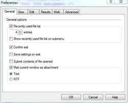
3) The ODS statement (Output Delivery System) modifies where output is sent and what output is included. The three statements below can be included in the housekeeping statements to alter the SAS 9.3 default behavior. These statements will cause the modifications described below. The “listing”, “noresults” and “graphics off” behavior can also be more permanently altered by specifying SAS preferences (e.g. Tools > Options > Preferences).
|
ODS listing; |
Causes TXT style output to be listed in the “OUTPUT” window. |
|
|
ODS noresults; |
Suppresses the default of HTML style output in the “RESULTS VIEWER” window. |
|
|
ods graphics off; |
Suppresses graphics produced by some SAS procedures for the HTML output. |
Text output was listed in the OUTPUT window in previous SAS versions. This is no longer the default. If “ODS listing” is not included, the “OUTPUT” window will remain empty.
4) The TITLE1 statement adds a title line to the top of every page of output. A TITLE2 and TITLE3 statements will add a second and third title line. Additional titles can be added up to TITLE9.
OTHER NOTES
- SAS does not distinguish between upper case letters or lower case letters in the program, either can be used. However, it does distinguish between upper and lower case in datasets, so the character strings “Carol”, “carol” and “CAROL” would be considered different values of the variable “name” in the program above.
- Comments: Additionally, you may add comments anywhere in your program either by beginning the statement with an asterisk (*) and ending it with a semicolon (;) or by beginning with /* and ending with */. These comments may be thought of as marginal notes, and will show in the program editor and log, but not in the output window.
- Shortcuts: F4: recalls text once the program editor; F5: directs you to the program editor; F6: directs you to the log; F7: directs you to the output; F8 or the “running man”: submits your program; Ctrl+E clears content in the current window. Also, highlighted text can be copied with Ctrl+C, cut with, Ctrl+X or pasted with Ctrl+V.
LAB POLICIES
- Eating, drinking and smoking are prohibited in the lab.
- You are required to attend the lab section in which you are registered.
- Regular attendance is expected in order for you to not miss materials distributed in lab and discussions of the assignments given in the lab.
- Unless otherwise instructed, remember to log off but not to turn the computer or the monitor off when you leave.
- Be sure to leave your workstation clean when you leave. Deposit all waste paper in the recycling boxes next to the printers.
- The software loaded on the workstations in the lab is licensed to the department. Copying of this software is a federal offense.
- Do not load any personal software or data files on the computers.
- Printing problems: If you submit a file to the printer, and a dialog box pops up asking to RETRY? or CANCEL? Select CANCEL, then resubmit the print job. If you are experiencing printing problems, seek help from the lab instructor.
- Printing materials in the lab are for EXST course use only.
LAB ASSIGNMENTS
- Each lab report should start with a header containing your name, student number, lab section and assignment number.
- Each lab reports should provide your answers to any questions (when applicable) and appropriate SAS output (only the parts that are relevant to your answers). You should use an editor like Word to prepare the relevant portions of the output file for your report. Make your report neat, to the point, and concise, ensuring that any tables, charts or plots are not disrupted by page breaks.
- Each lab report is worth 10 points. Lab reports are due at the beginning of the next lab. If your lab report is late, you will lose a point per class day (2 per week) after the due date.
- You should be able to complete all necessary computer work during the lab period. However, you may use rooms 11 and 44 any time it is open and not occupied by another class. Check the door of the lab for a schedule of times that the lab is available.
- You are allowed (in fact, encouraged) to work with other students while in the lab, but the lab report that you submit must be your own work.
- Saving your work: You should save your program often. You may save your work on the lab machine but you will not necessarily have the same machine every week. Also, if disc space gets low the files may be deleted. It is strongly recommend that you save your program to a flash drive, Tigerbytes or email yourself a copy.
Assignment 1 (Due next week)
For this week’s lab you will run the SAS program below. You may copy and paste the program.
Although you can do a temporary save to the TEMP directory on the machine you are on, we strongly recommend that you save your work to a flash drive or to tigerbytes. Save your work soon and often.
Include the optional text listed above and two title statements. Call the first TITLE1 and the other TITLE2.
For example:
Title1 ‘Your name here and section number’;
Title2 ‘Put something about the assignment here’;
Make sure the program runs correctly.
Things to note about the program for Assignment 1.
|
* comment ; |
The program contains explanatory comments which do not affect the program execution. These start with an asterisk and end with a semicolon. They may run across several lines. |
|
Title statements |
A “title1” followed by text in single or double quotes and a semicolon statement will place the quoted string at the head of each page. A “title2 statement would occur on the second line”. These occur on all pages unless another title1 or title2 statement is placed in the program. A new title2 quoted string would replace title2 but would not change title1. Additional titles can be added up to title9. |
|
proc sort; |
Examine the differences in the output for these two sorts. Be sure you understand why they are different and what occurs when you sort by more than one variable. |
|
proc univariate; |
This is an important procedure. I can be used to obtain most of the simple statistics that are of interest in the course, some of the basic tests of hypothesis and some calculations such as confidence intervals and tests of normality that will be discussed later. |
|
PROCs with BY |
Once that data is sorted, procedures can be run with a BY statement to produce separate output for the sorted categories. Study the sort by gender and univariate by gender in this program. |
 The “plot” option on the proc univariate produces some simple graphics. One of the
graphics is a “stem and leaf plot” that shows how the observations are
distributed. The other is a “box plot” that shows the relative distribution of
some of the statistics from the distribution. In a symmetric distribution the
mean and median would be on the same line (e.g. *– – + – –*). The observed
pattern suggests a slight negative skew.
The “plot” option on the proc univariate produces some simple graphics. One of the
graphics is a “stem and leaf plot” that shows how the observations are
distributed. The other is a “box plot” that shows the relative distribution of
some of the statistics from the distribution. In a symmetric distribution the
mean and median would be on the same line (e.g. *– – + – –*). The observed
pattern suggests a slight negative skew.
Note that when proc univariate is run with a BY statement, the procedure produces a side by side box plot to compare the levels of the variable (male and female in this case).
Questions from the assignment
A physician has collected data on the height, weight, and gender of her patients. She wants to characterize the data set, and to visualize any relationships that might exist. Use the program to obtain answers for the following questions:
a) What are the minimum and maximum values for the height for males?
b) What is the value of the mean for weight for males?
c) What is the average weight for females?
d) From the side by side box plots, is the first quartile for the males higher than the third quartile for females for height?
e) Is the first quartile for the males higher than the third quartile for females for weight?
For this assignment turn in your whole SAS log, but only that SAS output that is relevant to answering the questions above.
dm 'log;clear;output;clear';
options nodate nocenter ls=78 ps=55;
OPTIONS FORMCHAR="|----|+|---+=|-/\<>*";
ODS listing; ods graphics off;
title1 'Lab1, Problem 2, Your name, Lab section ';
title2 "EXST 7005 Assignment 1";
data people;
input gender $ height weight;
datalines;
m 63 125
m 76 195
f 62 109
m 75 186
f 67 115
f 60 120
m 75 205
m 71 185
m 63 140
f 59 135
f 65 125
m 68 167
m 72 220
f 66 155
;
proc sort data=people;
by gender;
run;
proc print data=people;
title3 "Raw data sorted only by gender";
run;
proc sort data=people;
by gender height weight;
run;
proc print data=people;
title3 "Raw data sorted by gender, height and weight ";
run;
proc univariate data=people; by gender;
title3 "Univariate procedure output done separately by gender ";
title4 "The analysis was done for two quantitative variables";
var height weight;
run;
quit;